.md .pdf

Contents

Minimum Spanning Trees

Drexel owns a number of buildings in Philadelphia. They want all the buildings to have direct fiber connections. They can lease fiber from Verizon. What is the lowest lease payment that connects all the buildings? Our goal is not to get the best connection between any two buildings, it is to make sure all the buildings are connect at a minimum cost to Drexel.

The solution is something called a Minimum Spanning Tree!

Imagine the following graph shows the monthly cost to rent each fiber wire between buildings.

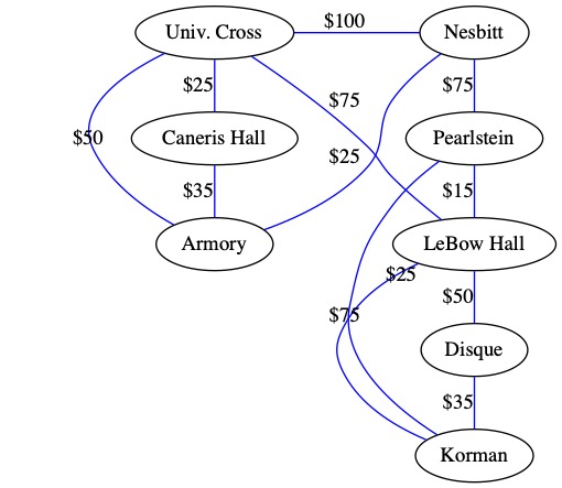
The best solution for Drexel is to pay $235 a month an lease the fiber lines highlighted below. Only renting these wires ensure that every building can talk to every other building and Drexel pays the minimum monthly fee. This helps Drexel keep tuition costs down.

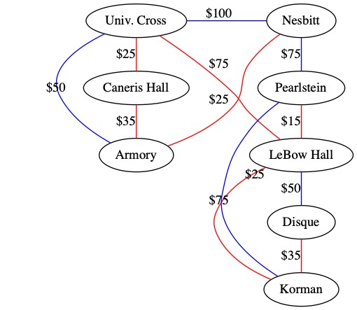
The result is a type of graph called a Minimum Spanning Tree or MST.

The name comes from the graph’s features.

• Tree: A graph that contains no cycles.

• Spanning: Reaching all nodes in a set or subset.

• Minimum: The smallest of all available options.

• MST: A tree with minimum total weight that spans all nodes.

Prim’s Algorithm

In 1830, Vojtech Jarnik discovered an algorithm to find the minimum spanning tree. This algorithm was not made famous until it was rediscovered by Robert Prim in 1957. Prim’s algorithm is described below.

Prim’s algorithm is a greedy algorithm. A greedy algorithm always choose the locally optimal option. After all decisions are made, we will have the Global Optimal option. Not all problems can be solved by using greedy methods.

The basic concept is that we start with 1 node in the MST. We select the minimum weight edge that connects to a node that is not in the MST. We keep doing this until every edge is in the MST.

We select the minimum weight cut between two sets of edges. The set containing the partially created MST and the set of nodes not currently in the MST.

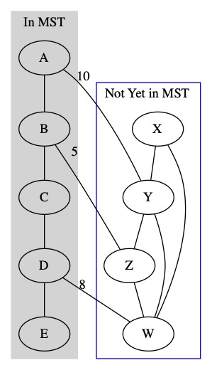
We keep repeating this process until we get every node into the MST.

Prim Walkthrough

We start with an initial graph. We want to find the MST of this graph.

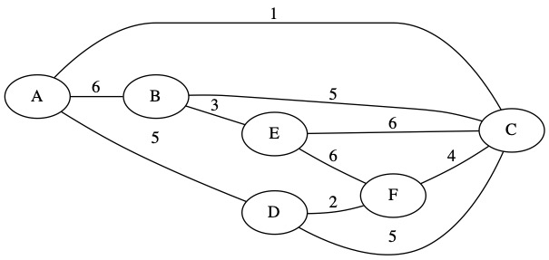
We also need to be given a starting node. This is the first node we will put into our partially complete MST set.

We will use node A as our starting node.

Since node A is our starting know, we also know about all it’s edge. We make a priority queue storing the edges we know about.

We also keep a set of nodes \(U\) with the nodes currently in the MST. Right now, only node A is in the MST. The edges are written as 3-tuples (weight, from, two). Since this is an undirected graph, we put the edge nodes in alphabetical order.

U = {A}
Known Edges in PQ: (1, A, C) (5, A, D) (6, A, B)

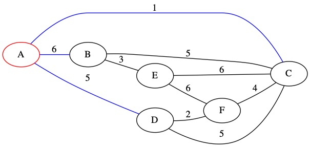
The smallest of our known edges is (1, A, C). It has weight 1. This edge connects node A which is in the MST to node C which is not currently in the MST.

We add this edge to the MST and add node C to our set. We also add all node C’s edges to the priority queue.

U = {A, C}
Known Edges in PQ: (4, C, F) (5, A, D) (5, C, D) (B, C, 5) (6, A, B) (6, C, E)

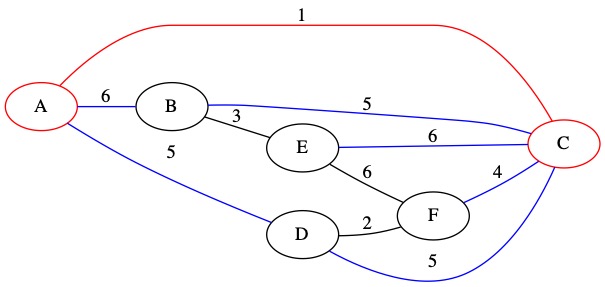
The smallest of our known edges is (4, C, F). It has weight 4. This edge connects node C which is in the MST to node F which is not currently in the MST.

We add this edge to the MST and add node F to our set. We also add all node F’s edges to the priority queue.

U = {A, C, F}
Known Edges in PQ: (2, D, F) (5, A, D) (5, C, D) (B, C, 5) (6, A, B) (6, C, E) (6, E, F)

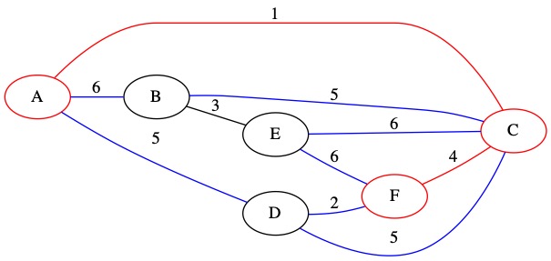
The smallest of our known edges is (2, D, F). It has weight 2. This edge connects node F which is in the MST to node D which is not currently in the MST.

We add this edge to the MST and add node D to our set. We also add all node D’s edges to the priority queue.

U = {A, C, F, D}
Known Edges in PQ: (5, A, D) (5, C, D) (B, C, 5) (6, A, B) (6, C, E) (6, E, F)

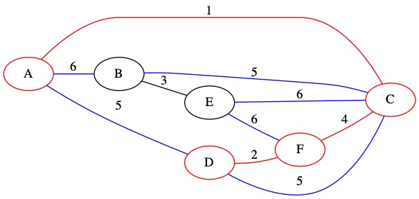
The smallest of our known edges is (5, A, D). It has weight 5. This edge connects two nodes that are already in the MST. We decide not to include it in the MST.

No changes are made to \(U\). The edge is removed from the priority queue.

U = {A, C, F, D}
Known Edges in PQ: (5, C, D) (B, C, 5) (6, A, B) (6, C, E) (6, E, F)

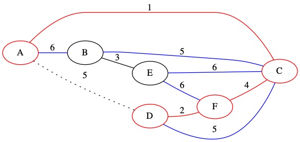
The smallest of our known edges is (5, C, D). It has weight 5. This edge connects two nodes that are already in the MST. We decide not to include it in the MST.

No changes are made to \(U\). The edge is removed from the priority queue.

U = {A, C, F, D}
Known Edges in PQ: (B, C, 5) (6, A, B) (6, C, E) (6, E, F)

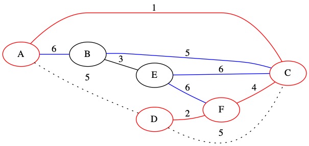
The smallest of our known edges is (5, C, B). It has weight 5. This edge connects node C which is in the MST to node B which is not currently in the MST.

We add this edge to the MST and add node B to our set. We also add all node B’s edges to the priority queue.

U = {A, C, F, D, B}
Known Edges in PQ: (3, B, E) (6, A, B) (6, C, E) (6, E, F)

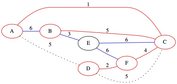
The smallest of our known edges is (3, B, E). It has weight 3. This edge connects node B which is in the MST to node E which is not currently in the MST.

We add this edge to the MST and add node E to our set. We also add all node E’s edges to the priority queue.

U = {A, C, F, D, B, E}
Known Edges in PQ: (6, A, B) (6, C, E) (6, E, F)

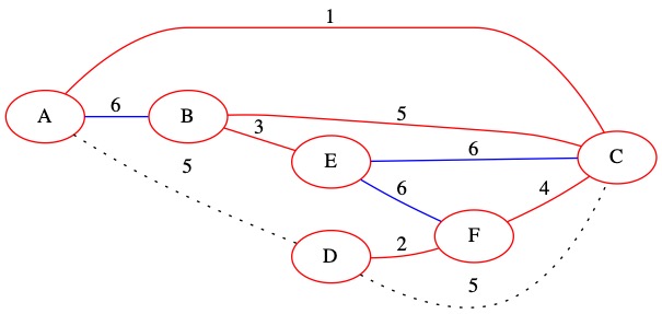
The smallest of our known edges is (6, A, B). It has weight 6. This edge connects two nodes that are already in the MST. We decide not to include it in the MST.

No changes are made to \(U\). The edge is removed from the priority queue.

U = {A, C, F, D, B, E}
Known Edges in PQ: (6, C, E) (6, E, F)

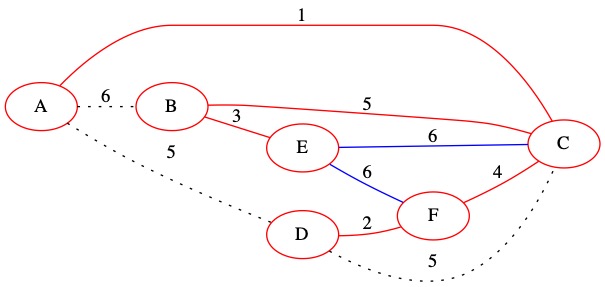
The smallest of our known edges is (6, C, E). It has weight 6. This edge connects two nodes that are already in the MST. We decide not to include it in the MST.

No changes are made to \(U\). The edge is removed from the priority queue.

U = {A, C, F, D, B, E}
Known Edges in PQ: (6, E, F)

The smallest of our known edges is (6, E, F). It has weight 6. This edge connects two nodes that are already in the MST. We decide not to include it in the MST.

No changes are made to \(U\). The edge is removed from the priority queue.

U = {A, C, F, D, B, E}
Known Edges in PQ: 

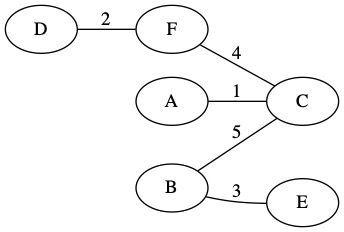
There are no edges left in the priority queue. That means we have created the MST. It is shown with only the tree edges below. The total weight of the MST is 15.

Prim Implementation

To implement Prim’s algorithm we start with an input graph and start node. We make a new empty graph by calling createAdjMatrix(). We will use this adjacency matrix to store the resulting MST. We fill in the graph with infinity on all edges except the diagonal which gets zeros using emptyGraph(MST, numNodes(G)).

We create a new empty set to store the nodes in the MST using Let set U  = newSet(). We also need to create an empty priority queue to use with Let PQ  = createEdgePQ().

We add the start node to our set with addToSet(start, U). We add all its edges to the priority queue using pushAdjEdges(PQ, G, start).

Since we know how many nodes exist, we can exist the loop when they are all in the MST. If we did not know how many nodes to expect, we would loop until the priority queue was empty.

At each iteration of the loop, we get the minimum edge from the priority queue. We check to see if it connects an edge in the MST to and edge that is not in the MST. If it does, we add it to the MST.

The algorithm is described below in code. We take advantage of the way Prim’s works to make sure the to from node one each edge is always the node that is already in the MST.

/*
    Prim's Algorithm for MST
    Returns a new Graph with only the MST edges
*/
Function Prim(Graph G, Node start)
    //Create an Empty Graph to store results
    Let MST = createAdjMatrix()
    //Start with all infinity values except diagonal
    emptyGraph(MST, numNodes(G))
    //Create a Priority Queue to Manage Edges
    Let PQ = createEdgePQ()
    //Use a Set to track our nodes
    Let U = newSet()
    //Initialize with Start Node
    addToSet(start, U)
    //Add Edges to Priority Queue that are adjacent to start node
    pushAdjEdges(PQ, G, start)
    //While we have not added all nodes to the set
    While countItems(U) != numNodes(G) do
        //Get the edge with the smallest weight
        Let e = minEdge(PQ)
        //If the to node is not already in our tree
        If not isInSet(toNode(e), U) then
            //Add edge to the MST Set
            addToSet(toNode(e), U)
            //Add Edge to the MST
            addEdge(MST, fromNode(e), toNode(e), weight(e))
            //Add both ways since Undirected
            addEdge(MST, toNode(e), fromNode(e), weight(e))
            //Update the Heap with newly found edges
            pushAdjEdges(PQ, G, toNode(e))
        End If
    End While
    //Return the MST Graph
    Return MST
End Function

Prim Analysis

Let us assume our graph has \(n\) nodes. This means the maximum number of edges is \(n^2\). To create our empty adjacency matrix takes \(O(n^2)\). We then loop over edges. The loop will run at most once for every edge in the graph. This means the loop will run at most \(n^2\) times. Within the loop, we are updating the heap. Heap inserts and deletes take \(O(\log_{2}(n))\). This means the loop will take a total of \(O(n^2 \log_2(n^2))=O(n^2 \log_{2} n)\) time to find the MST for a graph.

Kruskal’s Algorithm

At about the same time as Prim came up with his algorithm, another algorithm was also developed to find MST. Prim published in 1957 in Bell Systems Technical Journal. Kruskal published in 1956 in the Proceedings of the America Mathematical Society. Prim technically discovered his algorithm first, but Kruskal won the race to publish.

Kruskal’s Algorithm sorts the edges before starting instead of keeping a heap.

Each algorithm has advantages:

• Prim: You don’t need to know about all the edges before you start.

• Kruskal: If you can sort your edges quickly (with a library sort for example), you will get a nice speed advantage.

The basic concept of Kruskal’s Algorithm is that we start by sorting all graph edges. Then we loop over the edges until we make the MST. For each edge, we decide if it belongs in the MST or not.

Kruskal Walkthrough

Kruskal’s Algorithm needs to start with a graph as input. We can use the same graph as we used on Prim’s Algorithm. This means we should get a tree with the same weight at the end, but we will reach it a different way.

We start by making a list with all the edges. For this example, we will use 3-tuples (weight, from, to). Since this is a undirected graph ever edge can be used in both directions. We put the from/to nodes in alphabetical order for easy reading.

(6,A,B)
(5,A,D)
(1,A,C)
(3,B,E)
(5,B,C)
(6,C,E)
(4,C,F)
(5,C,D)
(2,D,F)
(6,E,F)

We use a sorting algorithm (like quicksort) to sort the edges in order by weight. We broke ties using alphabetical order, but that won’t matter to the algorithm.

(1,A,C)
(2,D,F)
(3,B,E)
(4,C,F)
(5,A,D)
(5,B,C)
(5,C,D)
(6,A,B)
(6,C,E)
(6,E,F)

Kruskal’s Algorithm needs this sorted list of edges. We can’t do anything without it. It has to be our first step.

Next, we make a collection of sets. We have one set for each node.

{A}, {B}, {C}, {D}, {E}, {F}

We will use these sets to determine

• if we are done the MST

• if there are any cycles

We are done making out MST when there is only 1 set left with all the nodes it in.

We are done initialization and we can start the loop. We look at each edge in our sorted list.

The first edge is (1, A C). This edge connects node A and node C. These edges are currently in two different sets. That means that this edge will not create a loop.

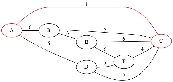
To keep track of this we union that two sets.

\( \begin{align} \{A\} \cup \{C\} =& \{ A, C \} \end{align} \)

Our collection of sets now has 4 sets instead of 5.

{A, C}, {B}, {D}, {E}, {F}

We also need to keep track of out Tree edges. We can call this set \(T\). These are the edges we want in the MST when we are done.

T = { (1, A, C)}

The next edge is (2,D,F). This edge also does not create a loop because node D and node F are in different sets. We will add this edge to the MST.

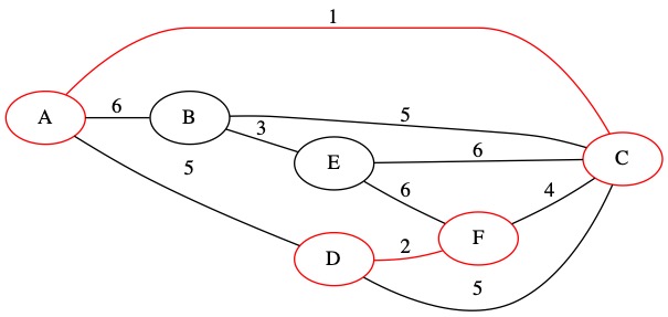
We union the two sets of nodes and add the edge to our set \(T\).

Collection of Sets = {A, C}, {B}, {D, F}, {E}
T= { (1, A, C), (2, D, F)}

The next edge is (3,B,E). This edge also does not create a loop because node B and node E are in different sets. We will add this edge to the MST.

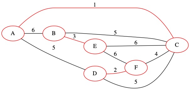
We union the two sets of nodes and add the edge to our set \(T\).

Collection of Sets = {A, C}, {B, E}, {D, F}
T= { (1, A, C), (2, D, F), (3, B, E)}

The next edge is (4,C,F). This edge also does not create a loop because node C and node F are in different sets. We will add this edge to the MST.

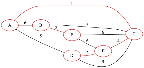
We union the two sets of nodes and add the edge to our set \(T\). Note that many nodes are merged in this step because \(\{A, C\} \cup \{D,F\} = \{A,C,D,F\}\). All four of these nodes now have paths to reach each other in the MST.

Collection of Sets = {A, C, D, F}, {B, E}
T= { (1, A, C), (2, D, F), (3, B, E), (4,C,F)}

The next edge is (5,A,D). This edge does create a loop. Both node A and node D are already in the same set. We chose not to use this edge.

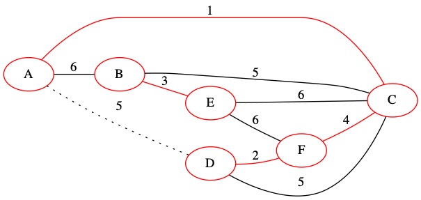
The sets do not change in this iteration.

Collection of Sets = {A, C, D, F}, {B, E}
T= { (1, A, C), (2, D, F), (3, B, E), (4, C, F)}

The next edge is (5,B,C). This edge does not create a loop. It connects two nodes that are in different sets.

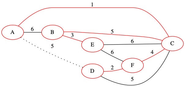
We update the sets to track our progress.

Collection of Sets = {A, C, D, F, B, E}
T= { (1, A, C), (2, D, F), (3, B, E), (4, C, F), (5, B C)}

The next edge is (5,C,D). This edge does create a loop. We do not add it to the MST.

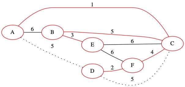
The sets do not need to be updated.

Collection of Sets = {A, C, D, F, B, E}
T= { (1, A, C), (2, D, F), (3, B, E), (4, C, F), (5, B C)}

The next edge is (6,A,B). This edge does create a loop. We do not add it to the MST.

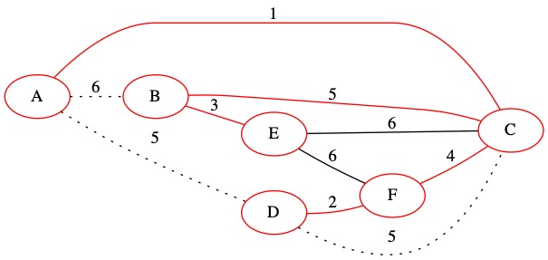
The sets do not need to be updated.

Collection of Sets = {A, C, D, F, B, E}
T= { (1, A, C), (2, D, F), (3, B, E), (4, C, F), (5, B C)}

The next edge is (6,C,E). This edge does create a loop. We do not add it to the MST.

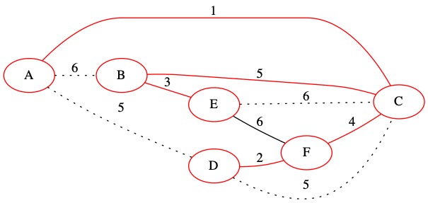
The sets do not need to be updated.

Collection of Sets = {A, C, D, F, B, E}
T= { (1, A, C), (2, D, F), (3, B, E), (4, C, F), (5, B C)}

The next edge is (6,E,F). This edge does create a loop. We do not add it to the MST.

The sets do not need to be updated.

Collection of Sets = {A, C, D, F, B, E}
T= { (1, A, C), (2, D, F), (3, B, E), (4, C, F), (5, B C)}

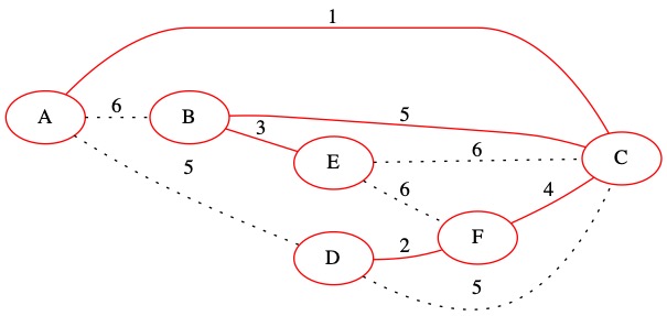
We have looked at every edge in the graph and decide if each is part of the MST or not. We can now simplify the graph by only drawing the MST edges. The total weight of this MST is 15.

Kruskal Implementation

To implement this algorithm, we need a place to store our MST edges. It makes sense to just use another graph to store the results. That way we can provide the graph as our result. We use a function createAdjMatrix() to return an empty adjacency matrix. Then we call a method on it emptyGraph(MST, numNodes(G)). This method makes the matrix have numNodes(G) nodes. It sets the diagonal of the matrix to 0 and fills all other spaces with infinity. This gives us a working graph to store the MST in. This could also be implemented with an adjacency list.

We make an array with all the edges in the graph using arrayOfEdges(G). Once we have the array, we can use Quick Sort to sort it.

We need to create a collection of sets. This is encapsulated into the function createSetCollection(numNodes(G)).

We now start the loop. For every edge in the edge list, we need to decide if it goes in the MST or not. We get an edge from the sorted lists and look at both sides. We check to see if they are in the same set or different sets using findSet(fromNode(e), S) != findSet(toNode(e), S).

If they are in different sets, then we add this edge to our MST. Since this is an undirected adjacency matrix, we add the edge to in both directions. We also union the two sets to avoid loops in the future union(S, fromNode(e), toNode(e)).

The full algorithm is provided below.

/*
    Kruskal's Algorithm for MST
    Returns a new Graph with only the MST edges
*/
Function Kruskal(G Graph)
    //Create an Empty Graph to store results
    Let MST = createAdjMatrix()
    //Start with all infinity values except diagonal
    emptyGraph(MST, numNodes(G))
    //Make an Array of All Edges
    Let EdgeList = arrayOfEdges(G)
    //Sort the Edges
    Quicksort(EdgeList)
    //Create a Collection of sets
    Let S = createSetCollection(numNodes(G))
    //Loop over all edges
    For i = 0, i < len(EdgeList), i++ do
        Let e = EdgeList[i]
        If findSet(fromNode(e), S) != findSet(toNode(e), S) then
            //Add to the MST
            addEdge(MST, fromNode(e), toNode(e), weight(e))
            addEdge(MST, toNode(e), fromNode(e), weight(e))
            //Merge the Sets
            union(S, fromNode(e), toNode(e))
        End If
    End For
    //Return the MST Graph
    Return MST
End Function

Analysis

In the worst case situation, ever single edge has a value. That means if we have \(n\) nodes, there are \(n^2\) edges. Making the empty adjacency matrix takes \(O(n^2)\) work. Using quicksort to sort the edges takes \(O(n^2 \log_{2} n)\).

\( \begin{align} O\left( (n^2) \log_{2}(n^2)\right) = O\left( n^2 \log_{2} n\right) \end{align} \)

The loop will run at most \(O(n^2)\) times. The only question is how long the findSet commands will take. If they are linear time, that will be \(O(n^3)\). If we can implement the findSet in constant time, then this loop is only \(O(n^2)\). We can implement these set operations in constant time. See the section on managing sets to see some ways to implement sets efficiently.

This means the deciding factor in the runtime is the sort itself. This gives Kruskal’s Algorithm a runtime of \(O(n^2 \log_{2} n)\).

A Set Structure for Kurskal

The only part of this we don’t already have a data structure for is the collection of sets. This is called a Disjoint Set Collection. We need an efficient implementation of Kruskal will be slowed down.

We make a forest of trees for the collection of sets. For each node in the graph, we will store three things.

• The node’s value

• The parent of the node

• The rank of the node

The rank will approximate how many values are in the set. When we union, we will move values from the smaller set to improve efficiency. The root of any tree will be used as the name of the set. It a set has node 5 as it’s root, we will call it set 5.

We can build this structure from an array of trees. In each position in the tree, we store the parent of the node \(p\) and the rank of the node. We create an array such that \(A[x]\) contains all information about node \(x\).

Since we will already know the edge we are looking at, we can find anything we need in this array quickly and efficiently.

To make a new set, we create an array. Every node’s parent is itself. It is in a set alone. Every node has a rank of 0.

Function makeSet(A,x)
    A[x]'s p = x
    A[x]'s rank = 0
End Function

To make the whole forest we just iterate over this function.

Function makeForest(n)
    A = array with n positions
    For i = 0, i < n, i++ do
        makeSet(A,i)
    End For
End Function

To find a set, we start at the node requested. We follow the parent indexes until we find a node who is it’s own parent. This denotes it as the root of the set. The set name is the node that is the root of the tree.

While we are doing this, we apply an optimization called path compression. Once we find out that name of the set, we update out parent index to point directly to the root node. This way, next time we search there is only 1 step to the root.

Function findSet(x, A)
    //Only search if we are not root
    If(x != A[x]'s p ) then 
        //Find our parent's set
        Let setID = findSet(A[x]'s p,A)
        //Compress the path
        Let A[x]'s p = setID
    End If
    Return A[x]'s p
End Function

The union operation merges all the elements in two sets together. We point the root of the smaller set at the larger set. A helper function is used here.

Function union(x,y,A)
    link(findSet(x), findSet(y), A)
End Function

The link function updates the root pointer in the set with the smaller number of elements. Later, path compression will shrink longer trees.

Function link(x,y,A)
    If A[x]'s rank > A[y]'s rank then
        A[y]'s p = x
    Else
        A[x]'s p = y
        If A[x]'s rank == A[y]'s rank then
            A[y]'s rank = A[y]'s rank + 1
        End If
    End If
End Function

For practical purposes finding and executing a union on \(m\) sets will take \(O(m)\).The set operations will not increase the running time of the algorithm since it is already linear time. The real running time for merging \(m\) sets of \(n\) total things is \(O(m \alpha(n))\). For practical purposes, \(\alpha(n) \le 4\), we can just pretend it is 4. As long as the number of elements in set is less than about \(10^{80}\) we have \(\alpha(n) \le 4\).

Traveling Salesperson Problem

The **Traveling Salesperson Problem is defined as follows.

Given a list of locations and distances between locations, what is the shortest possible route that visits each city exactly once and returns to the starting point?

This is important in many real world situations.

• Deliver mail and return to post office

• Stop at every capital on a political campaign and end up at home

• Visit factories for inspection and return to home office

Assume we want to solve the TSP for \(n\) cities. This problem is NP-Hard, in the worst case we need to do at least \(O(2^n)\) work. Trying all possible combinations is \(O(n!)\). This will never work for large sizes of \(n\). It would take the computer far to long to brute force the correct answer.

\[ \begin{align*} \lim_{n=\infty} \frac{n!}{2^n} = \infty \end{align*} \]

The best know solution is the Held-Karp Algorithm. This can find the exact solution in \(O(n^2 2^n)\). Better than \(O(n!)\) but still to slow for practical problems.

Why is TSP so hard? Imagine you are given a route of stops and told it is the shortest path. How would you be sure? The only way to know is to try all possible alternatives. Unlike in MST, local best decisions don’t help find the global best solution. It might be better to start at a further location to improve the round trip total.

A MST does tell us something about the TSP solution.

An MST is always smaller then the TSP path. It does not have a cycle, so at least 1 edge is needed to return to the start. The MST must have a lower weight than the best TSP solution.

Imagine we have already found an MST solution using either Prim or Kruskal. What if we just take every edge twice? We will go in a circle that takes us to every point and ends at the starting point.

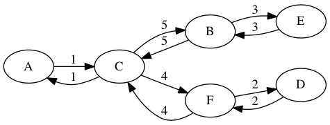
This may not be the optimal solution, but it does give us a cycle through all the nodes. Visiting every node twice gives us a path for the TSP, but it might not be optimal. We can predict that the TSP solution must be less than or equal to double weight of the MST.

Give a MST, we can conclude the following about the TSP solution.

\[ \begin{align*} w(MST) < w(TSP) \le 2*w(MST) \end{align*} \]

The MST can be used to approximate the solution to the TSP. Find the MST and take all edges both directions. This path is at worst double the TSP path. We can then search the MST using a DFS to try and find shortcuts. We might not find them all, but we will get a solution. We cannot be sure we will get the optimal solution, but it cannot be worse than double. This is a reasonable approximation since we know the exact solution is to difficult to compute directly.

We start with a full graph (all possible edges) between the locations. The graph must satisfy the Triangle Inequality. This means that dist(x,y) < dist(x,z) + dist(z,y). The direct path is always shorter then the two edges. The triangle inequality will hold for real world maps.

First, we find the MST. In this example, we used Prim’s Algorithm starting at node \(A\). The total weight is 7.

We now walk the MST in a cycle and look at what nodes we see. The order we walk through the nodes is A,B,C,B,A,D,A. The total length of this path is 14. We could implement this walk using a DFS.

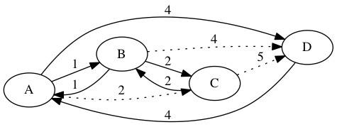
We remove duplicated nodes by using direct edges when possible. We replace the subpath C,B,A,D with the single edge C,D. The new walk is A,B,C,D,A. It has a total length of 12. If no direct way to shorten duplicates, then we leave the duplicates in the path.

We have found an approximation of the TSP solution. This path can be used to visit every node and return home. It may not be perfectly optimal, but we know in the worst case it is double optimal.

• Best Case: Solution is the optimal path for TSP

• Worst Case: Solution is 2*(shortest path)

The Triangle Inequality means this will never be worse then double the shortest path.

The algorithm is described below.

Function approxTSP(Graph G, Node a)
    Let T = prim(G,a) //Or Kruskal
    Do a full walk of T using DFS
    Reduce to a preorder walk (Remove unnecessary duplicates)
    Add/Remove edges to make MST match preorder walk if possible
    Return TSP Path
End Function

Approximate Runtimes:

• Find MST takes \(O( E \log_{2} V)\)

• A full walk (DFS/BFS) takes \(O(E+V)\)

• Removing Duplicates is \(O(E)\)

• Attempting to shorten the paths is \(O(E)\)

The deciding factor is finding the MST at \(O(E \log_{2} V)\). We already know how to do that! This is far more efficient than brute force \(O(V!)\) or Held-Karp Algorithm solves in \(O(V^2 2^V)\).

Are you willing to take a less optimal solution to save time?

The approximation is so much faster it can be used practically.

Assuming a full graph \(E=V^2\) the table below shows approximate work required.

Number Nodes	MST Approx	Held-Karp	Brute Force
5	58	800	120
10	332	102,400	3,628,800
25	2,903	\(2.09 * 10^{10}\)	\(1.55 * 10^{25}\)
50	14,109	\(2.81 * 10^{18}\)	\(3.04 * 10^{64}\)
100	66,439	\(1.26 * 10^{34}\)	\(9.33 * 10^{157}\)

There is an entire field of computer science dedicated to approximation algorithms. These are problems we know are \(O(2^n)\) or worse in the best know algorithm. Since solving the problem is to hard for practical purposes, we instead try to get a good enough solution faster.

previous

Breadth First Search

next

What is a Language?