Sorting Data¶

It is very useful to have organized data. We frequently run into problems that are easier to solve if the data is sorted. We already saw this with Binary Search. Think of all the different places you see data displayed. Keeping it in a sorted and well organized manner is crucial.

Normally, we don’t even realize how much sorting happens around us. This is because computers are really amazing at sorting. It is such a fundamental problem in computer science that we tend to forget about it. Doesn’t every programming language know how to sort?

Understanding how sorting works is a key theoretical concept. If you want to sort an array of integers, any language will happily do it for you. What happens when you need a custom sorting on data used in a program? Something that won’t be useful to anyone else. Understanding how sorting works allows us to make and modify existing sorting tools.

Comparison Sort¶

The most common sort is called the comparison sort. A comparison sort is just a sort that can be done by comparing values.

We have some function that can take two elements and tell us

True: they are in correct order
False: they are not in correct order

Since this comparison is so general, it is very easy to modify these algorithms to sort different things. To sort numbers, the comparison would be $a < b$.

It is possible to make more efficient algorithms with additional information. The more information we need, the more specialized the algorithm becomes. If we know we are sorting letters into alphabetical order, there any many improvements we can make. We know the smallest and largest letter. We know how many letters there are. This can provide more efficient algorithms, but they will be specialized for only letters.

Basics of Comparison Sorting¶

To sort an array using Comparison sorting there are a few requirements.

An array of data to sort
The size of the array must be known.
We must have a boolean comparison operation.
We must be able to swap elements in the array.

We need to be able to swap. If two values cannot be swapped, then it is impossible to sort efficiently. We would need to constantly create new arrays and move values.

The basic swap function is given below.

Function swap(array A, x int, y int)
    Let temp = A[x]
    A[x] = A[y]
    A[y] = temp
End Function

With these tools, we can build multiple comparison sorting algorithms.

Perfect Sorts¶

What would the perfect comparison sorting algorithm look like? The answer to this question will give us insight into how good or bad each sorting algorithms works.

We have an array with $n$ elements. We want to ask the minimum set of questions to determine the right ordering to put the numbers.

We can look at this question and determine what the minimal number of questions would be. This will give us a target to compare each of our algorithms to.

Trivial Cases¶

There are two trivial cases. In these cases, there are so few numbers the answer is obvious.

One element is sorted.
Two elements are trivial to sort.

To sort one element, we don’t have to do anything. One element must be sorted already. There is nothing that can be in the wrong place.

Function sort1(array A)
    Return
End Function

When sorting two elements, we compare them both. They are either in the correct order of need to be swapped.

Function sort2(array A)
    If A[0] > A[1] then
        swap(A, 0, 1)
    End If
End Function

Perfect Sort Three¶

Sorting three elements is the first non-trivial size.

Let us imagine an array with three numbers $[a,b,c]$. We will use letters as placeholders. These can be any values.

There are many questions we can ask: $a < b$, $a < c$, $b < c$, etc. We don’t need to ask every possible question. For example, if we determined $(a < b) = \text{True}$ and $(b < c)=\text{True}$ it would be pointless to ask $a < c$. We can determine that answer from the previous two.

There are $6$ permutations of three values.

$[a, b, c]$
$[a, c, b]$
$[c, a, b]$
$[c, b, a]$
$[b, a, c]$
$[b, c, a]$

Every time we ask a questions, we determine some permutations are impossible. By repeatedly asking questions, we narrow down the options to a single correct permutation.

What questions should we ask? This will determine how well the algorithm works.

We could ask $a < b$. There are three permutations where this is true and three where it is false.

$[a, b, c]$ $a < b$ is True
$[a, c, b]$ $a < b$ is True
$[c, a, b]$ $a < b$ is True
$[c, b, a]$ $a < b$ is False
$[b, a, c]$ $a < b$ is False
$[b, c, a]$ $a < b$ is False

Let us assume that $a < b$ is True, we only have three possible permutations to worry about. It is impossible for the others to be the correct sorting.

$[a, b, c]$
$[a, c, b]$
$[c, a, b]$

We can ask a second question $b < c$. If the answer is true, then we are done. There is only one permutation that makes sense $[a,b,c]$.

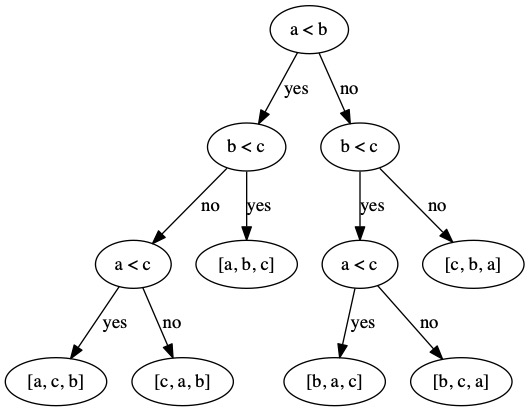
If $b < c$ is false, we have narrowed it down to two choices. We can ask $a < c$. If true then the sorting is $[a, c, b]$. If $a < c$ is false, then the sorting is $[c, a, b]$.

Using either two or three comparisons, we sorted the list.

We can make a decision tree that shows how the permutations are narrowed down.

Perfect Sort Three

We can also implement the decision tree as a function

Function sort3(array ARRAY)
    //This code ONLY works for 3 elements
    //Assign values to names
    Let a = ARRAY[0]
    Let b = ARRAY[1]
    Let c = ARRAY[2]
    //Comparison 1
    If a < b then
        //Comparison 2
        If b < c then
            ARRAY[0] = a
            ARRAY[1] = b
            ARRAY[2] = c
        Else
            //Comparison 3
            If a < c then
                ARRAY[0] = a
                ARRAY[1] = c
                ARRAY[2] = b
            Else
                ARRAY[0] = c
                ARRAY[1] = a
                ARRAY[2] = b
            End If
        End If
    Else
        //Comparison 2
        If b < c then
            //Comparison 3
            If a < c then
                ARRAY[0] = b
                ARRAY[1] = a
                ARRAY[2] = c
            Else
                ARRAY[0] = b
                ARRAY[1] = c
                ARRAY[2] = a
            End If
        Else
            ARRAY[0] = c
            ARRAY[1] = b
            ARRAY[2] = a
        End If
    End If
End Function

We can conclude that the absolute best solution to sorting three items is 3 comparisons. Some sequences will only take 2 comparisons, but we can’t do better than 3 in other cases. There is just no way to learn enough about the sequence without that third question.

Analysis of the Perfect Sort¶

The exact comparisons needed are known for values of $n=1$ to $n=11$. There are algorithms published for $n=12$ to $n=22$, but not all have been proven optimal [Wikipedia contributors, 2020]. For example, the best know solution for $n=22$ is 71 comparisons, but in theory it should be possible in 70 comparisons [Peczarski, 2004].

How can we estimate the best solution?

We can determine the number of possible permutations of an array. If an array has $n$ elements, then it will have $n!$ permutations. Optimally, each comparison will eliminate exactly half the possible permutations.

How many times can you divide $n!$ in half until only one element is left?

$ \begin{align} 1=& \frac{n!}{2^k} \\ 2^k =& n! \\ k =& \log_2(n!) \end{align} $

We need to do $\log_2(n!)$ comparisons. This probably won’t be an integer, so we can round up $\lceil \log_2(n!) \rceil$.

$\lceil \log_2(3!) \rceil = \lceil 2.58\cdots \rceil = 3$
$\lceil \log_2(5!) \rceil = \lceil 6.9\cdots \rceil = 7$
$\lceil \log_2(22!) \rceil = \lceil 69.92\cdots \rceil = 70$
$\lceil \log_2(100!) \rceil = \lceil 524.76\cdots \rceil = 525$

In the real world, it would not be worth anyone’s time or effort to find the perfect 525 comparisons to sort 100 elements. We want to come as close as possible. These bounds can give us a target for our implementations.

What Big Oh class do we want our algorithms to fall in?

$ \begin{align} \lceil \log_2(n!) \rceil =& O( n \log_2(n)) \end{align} $

If we can find an algorithm that sorts in $O( n \log_2(n))$, we will be within a constant multiplier of the perfect solution.

Sort Five Elements¶

Given an array with exactly 5 elements, we can sort it using a maximum of seven comparisons.

This is what we expect because $5!=120$ and $\log_2(120)=6.9...$.

This code is $O(1)$, but it is only useful for an array with exactly $5$ elements. In short, this kind of perfection is not worth the programmer’s effort. It does sort with the optimal number of comparisons.

In the best case, this algorithm does 6 comparisons. In the worst case, it does 7 comparisons.

This solution helped get Howard B. Demuth his Ph.D. in 1956 [Demuth, 1956].

Function sort5(A []int) {
    //Only works for exactly 5 elements
    //First Comparison
    If A[0] > A[1] then
        swap(A, 0, 1)
    End If
    //Second Comparison
    If A[2] > A[3] then
        swap(A, 2, 3)
    End If
    //Third Comparison
    If A[1] > A[3] then
        swap(A, 0, 2)
        swap(A, 1, 3)
    End If
    //Fourth Comparison
    If A[1] > A[4] then
        //Fifth Comparison (Path A)
        If A[0] > A[4] then
            swap(A, 3, 4)
            swap(A, 1, 3)
            swap(A, 0, 1)
        Else
            swap(A, 3, 4)
            swap(A, 1, 3)
        End If
    Else
        //Fifth Comparison (Path B)
        If A[3] > A[4] then
            swap(A, 3, 4)
        End If
    End If
    //Sixth Comparison
    If A[2] > A[1] then
        //Seventh Comparison (Path A)
        If A[2] > A[3] then
            swap(A, 2, 3)
        End If
    Else
        //Seventh Comparison (Path B)
        If A[0] > A[2] then
            swap(A, 2, 1)
            swap(A, 1, 0)
        Else
            swap(A, 2, 1)
        End If
    End If
End If

Sorting Algorithms¶

Let us review the four sorting algorithms we have already seen. We can now compare them to the imaginary perfect sort. There is also one more algorithm that we will see later in the term here called Heap Sort.

Algorithm	Average Runtime	Worst Runtime	Worst Case Memory Usage
Bubble Sort	$O(n^2)$	$O(n^2)$	$O(1)$
Insertion Sort	$O(n^2)$	$O(n^2)	$O(1)$
Merge Sort	$O(n \log n)$	$O( n \log n)$	$O(n)$
Quick Sort	$O(n \log n)$	$O(n^2)$	$O(n)$
Heap Sort	$O(n \log n)$	$O(n \log n)$	$O(1)$

Note

There are optimizations that can get Quick Sort’s memory to $O(\log n)$ in the worst case instead of just in the average case.

We determined the the perfect sort would be in the class $O(n \log n)$. Two of the algorithms we have already seen, Merge Sort and Quick Sort, fall in the same asymptotic class as the perfect sort would. We may not be perfect, but we are at least in the same ballpark.

Algorithm	Average Runtime	Worst Runtime	Worst Case Memory Usage
Bubble Sort	\(O(n^2)\)	\(O(n^2)\)	\(O(1)\)
Insertion Sort	\(O(n^2)\)	$O(n^2)	\(O(1)\)
Merge Sort	\(O(n \log n)\)	\(O( n \log n)\)	\(O(n)\)
Quick Sort	\(O(n \log n)\)	\(O(n^2)\)	\(O(n)\)
Heap Sort	\(O(n \log n)\)	\(O(n \log n)\)	\(O(1)\)

Algorithmic Foundations of Computer Science

Sorting Data

Contents