Binary Search Trees
Contents
Binary Search Trees
Tree Arity
The arity of a tree is the maximum number of children any node can have. This is a maximum. A node can always have less children, but never more.
The arity of a tree can always be described as M-ary where \(M\) is the maximum number of children. A few common arities have special names.
Unary Tree has at most 1 child. This is a Linked List. A 1-ary tree.
Binary Tree has at most 2 children. A 2-ary tree.
Ternary Tree has at most 3 children. A 3-ary tree.
The example in the previous section was a Ternary or 3-ary tree.
BST Structure
A Binary Search Tree (BST) is a Binary Tree with special properties that make it efficient to search.
A BST is designed to allow efficient addition/removal of values and still be able to binary search the values. It is a ordered tree. The nodes are kept in a strict order to ensure easy searching.
This makes a BST efficient to search, but also efficient to change.
The ordering of a BST is strictly defined.
The left child and all it’s proper descendants must be less than the parent.
The right child and all it’s proper descendants must be greater than the parent.
Note
What happens to equal values? If you only ever need to search, then there is no reason to keep duplicates. If the duplicates matter, pick a side and be consistent.
Searching for Items
The two most basic features are inserting values and searching. If we can’t insert any values, there is no point in searching. We need to build the structure before we can search it.
Insertion
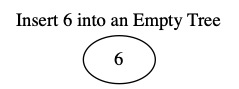
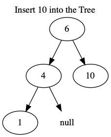
To make a BST we start with an empty tree. Each node is inserted such that the two properties are meet.
The algorithm for inserting a target value can be summarized as:
If the location is empty then create a new node and store target value.
If the location is not empty then compare node value to the target value.
If values are the same then make no changes.
If node value is larger then insert recursively on left.
If node value is smaller then insert recursively on right.
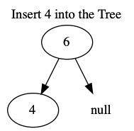
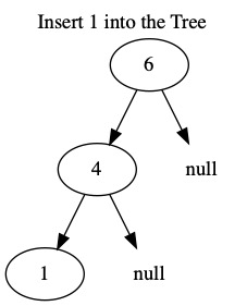
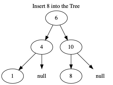
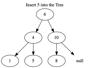
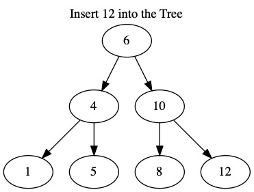
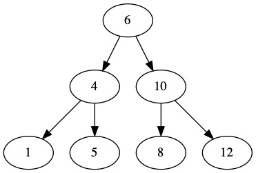
The following images insert the values \(6, 4, 1, 10, 8, 5, 12\). When building a tree, the order we insert the values matters.
Search
To search for a value, we can take advantage of the tree’s strict ordering. Searching is a boolean question. We search for a target value in the tree. We want to return true if it is found and false otherwise.
We always start at the top. If the target value is smaller than the root then we search the left side of the tree recursively. If the target value is larger than the root then we search the right side of the tree recursively. If the target value is equal to the root then we can return true. If the target value is never found then we can return false.
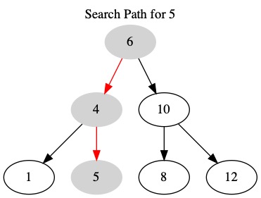
If we want to search for 5, we need to do three comparisons
Compare 5 to the root (6). Go left because 5 is smaller than 6.
Compare 4 to left child (4). Go right because 5 is larger than 4.
Compare 5 to right child (5). We found the target. Return true.
Implementation
To implement our BST, we need a node structure. The node has a value and pointers for the left and right values.
//Node is a Data Structure to hold a binary tree node.
struct Node {
    //Store the Node's Value
    int value
    //Pointer to Left subtree
    Node* left
    //Pointer to Right subtree
    Node* right
}
A tree is just a bunch of nodes starting at the root. We only need to know where the root is. We can find everything else by following pointers. The tree has it’s own structure.
//BST is a Data Structure to hold a Binary Search Tree
struct BST {
    //We need a pointer to the Root node
    Node* root
}
We can’t create anything if we can’t make an empty tree. The following function just allocates memory for an empty tree.
//MakeTree creates a new empty binary search tree
Function MakeTree()
    //Allocate a new BST and get pointer
    T = allocateBST()
    //Set the root to be empty
    T's root is null
    //Return pointer to tree
    Return T
End Function
At this point, we have enough code structure to start building algorithms. All tree algorithms will be recursive. We will make two functions for each feature. One that programmers user, these always start at the root. We will have a second function that can be executed at any node. These will be used internally for implementation.
A user of our data structure wants to find a value in the tree.
//Find searches for target value in tree
Function Find(int value, BST* Tree)
    //Start recursive search at the root
    return findInTree(value, Tree's root)
End Function
We just execute the recursive implementation starting at the root. The recursive implementation compares to values and moves left or right. It will either find the target or run out of options.
//findInTree searches nodes for a value
Function findInTree(int value, Node* currentNode)
    //If the node is empty then nowhere to look.
    If currentNode is null then
        Return false
    End If
    //If the value is the current node, we found target
    If currentNode's value == value then
        Return true
    End If
    //Otherwise, compare and search one side.
    If currentNode.value > value then
        //Node is to big, search left
        Return findInTree(value, currentNode's left)
    End If
    //Node is to small, search right
    Return findInTree(value, currentNode's right)
End Function
We need to do a similar thing to insert. The user of our data structure just wants to insert a value.
//Insert inserts a new value into the tree (if not already in it).
Function Insert(int value, BST* Tree)
    //This might change the root node
    Tree's root = insertValue(value, Tree's root)
End Function
We need to deal with updating pointers. We need to search the tree for a place to put the value. Then we need to update all the pointers to account for the new node.
Note
We won’t know where in the recursion the new pointers appear. Every call needs to return pointers. Some will be unchanged, but we won’t know that until the return.
//insertValue recursively searches for a location to insert the value.
//It returns a pointer to the updated node.
Function insertValue(int value, Node* currentNode)
    //If we are an empty position, create a new node
    If currentNode is null then
        Let newNode = allocateNewNode()
        newNode's value = value
        newNode's left = nil
        newNode's right = nil
        Return newNode
    End If
    //If the value is found, ignore it
    If currentNode's value == value then
        Return currentNode //No Changes
    End If
    //Recursively update either left or right side
    If currentNode's value > value then
        //Insert and update on left
        currentNode's left = insertValue(value, currentNode's left)
        //Return updated node
        Return currentNode
    End If
    //Insert and update on right
    currentNode's right = insertValue(value, currentNode's right)
    //Return updated node
    Return currentNode
End Function
Tree Information
Normally, we want to do more than just search. We want to ask questions about the tree. We may even need to display the tree.
Get the Root
It is sometimes helpful to get direct access to the pointers. This function returns the root node pointer.
//GetRoot returns the root node of the tree
Function GetRoot(BST* T)
    Return T's root
End Function
Height
Finding out the height of the tree is very important. It allows us to determine if the tree is empty or not. It also allows us to determine if it has become unbalanced. A tree with no values has a height of \(-1\).
We need a public function that starts at the root.
//Height tells you the height of the tree
Function Height(BST* T *BST)
    //The tree height is the node height of the root
    Return nodeHeight(T's root)
End Function
We can implement a recursive function to find the height of a node. Since the height of the root is the height of the tree, this is used as a helper to find the tree height.
//nodeHeight determines the height of a node
Function nodeHeight(Node* currentNode)
    If currentNode is null then
        Return -1
    End If
    Let leftHeight = nodeHeight(currentNode's left)
    Let rightHeight = nodeHeight(currentNode's right)
    If leftHeight > rightHeight then
        Return leftHeight + 1
    End If
    Return rightHeight + 1
End Function
Displaying the Tree
It is great to have nice graphics of the tree. In practice, this will normally not be possible. In a text-based program, we still need a way to visualize the tree. This is crucial for debugging.
There are three common methods for printing out a tree.
Preorder: Print Node, Print Left Children, Print Right Children
Postorder: Print Left Children, Print Right Children, Print Node
Inorder: Print Left Children, Print Node, Print Right Children
Examine the following tree as an example.
For preorder, we start with the node’s value, then recursively deal with the left and right. When we get to empty positions, we print N for null. The following example shows how the recursion builds the text to display. Parenthesis are added to show grouping in intermediate steps.
Start Preorder at Root
Print Node, Print Left Children, Print Right Children
6 (Node LC RC) (Node LC RC)
6 (4 (Node LC RC) (Node LC, RC)) (10 (Node LC RC) (Node LC RC))
6 (4 (1 N N) (5 N N)) (10 (8 N N) (12 N N))
6 4 1 N N 5 N N 10 8 N N 12 N N
In postorder, we put the root value at the end instead of the beginning.
Start Postorder at root
Print Left Children, Print Right Children, Print Node
(Node LC RC) (Node LC RC) 6
((Node LC RC) (Node LC RC) 4) ((Node LC RC) (Node LC RC) 10) 6
((1 N N) (5 N N) 4) ((8 N N) (12 N N) 10) 6
1 N N 5 N N 4 8 N N 12 N N 10 6
With inorder, we put the root value in between the left and right side. This gives us a sorted list of values! It doesn’t tell us as much about the tree structure as the other two.
Start Inorder at root
Print Left Children, Print Node, Print Right Children
(LC Node RC) 6 (LC Node RC)
((LC Node RC) 4 (LC Node RC)) 6 ((LC Node RC) 10 (LC Node RC))
((N 1 N) 4 (N 5 N)) 6 ((N 8 N) 10 (N 12 N))
N 1 N 4 N 5 N 6 N 8 N 10 N 12 N
Using all three of these prints together, it is easy to rebuild the structure of the tree on paper.
Deleting Values
Deleting a value from the tree is the most complicated operation. We need to keep all the properties of the BST, but we also want to minimize our changes. This requires a more complex algorithm.
Removing Values
The easiest node to remove is a leaf. It has no children. We just need to update the parent to know the child has been removed.
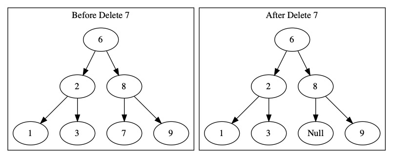
It is also easy to delete a node with only one child. We just update the parent to point directly to the child. The node in the middle is gone.
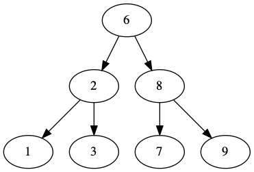
The challenge comes when we want to delete a node with two children. We need to keep the tree properties. We want to delete 6 from the following tree. Is has many children. This is the worst case situation.
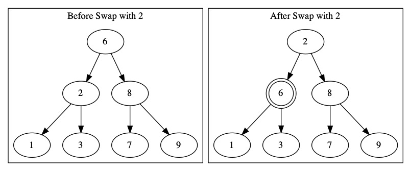
We already know leaves are trivial to delete. Could we swap 6 into a leaf? That would make it easier to delete. If we swap it with 2, the tree doesn’t get any easier to work with. The same thing happens with 8. We can’t swap with an internal node. It won’t make the problem any easier.
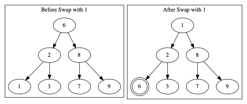
We could swap with values 1 or 9. They would make it easy to delete 6. They introduce a different problem. They break other nodes in the tree. These swaps will cause even more work for us. We will need to fix the tree.
There are two values that can be swapped with the root. The maximum of the left side and the minimum of the right side.
Swapping with the value 3 keeps everything else in the tree correct. It also makes 6 a leaf. We can easily delete 6 after this swap.
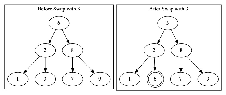
The same thing happens if we swap with 7. The tree structure holds.
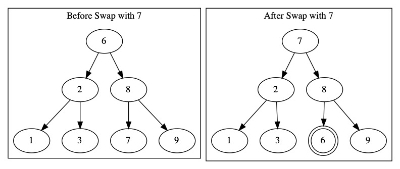
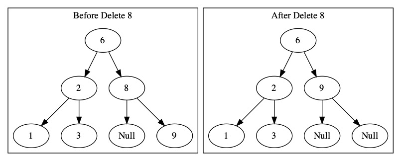
We can use either of these, but we need to be consistent. When we delete an node with two children, we swap it to a easier position. We will use the minimum of the right side.
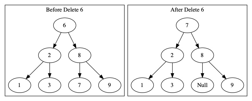
The minimum of the right side must be an easy to delete value and also a root replacement. Since it is the minimum it has either 0 or 1 child. These are both easy to delete. It cannot have two children and also be the minimum. It’s left child would be smaller.
The minimum of the right side is larger than everything on the left side and also smaller than everything on the right side except the root. Since the root is being deleted, this node will fit in the root position without breaking the tree properties.
Finding the Min
The minimum value is a binary search tree is reasonably easy to find. If there is a smaller value, it is always to the left. We move left until we run out of left children. The node we end on must be the minimum. There is nothing smaller than it.
The minimum of the entire tree starts searching at the root.
//Min determines the minimum value in the tree
Function Min(BST* Tree)
    Return findMin(Tree's root)
End Function
We can find the minimum of any node by searching recursively starting at that node. We just go left until we run out of left children.
//findMin finds the min starting at any node
Function findMin(Node* currentNode)
    //Return -1 for error
    If currentNode is null then
        Return -1
    End If
    //If no left child then at min
    If currentNode's left == nil then
        Return currentNode's value
    End If
    //Otherwise keep searching
    Return findMin(currentNode's left)
End Function
Delete Implementation
At the top level, we delete a value from the root of the tree.
//Delete removes a value from the tree
Function Delete(int value int, BST* Tree)
    Tree's root = deleteValue(value, Tree's root)
End Function
We need to search the three for the value we want to delete. The function deleteValue searches the tree. When it finds the target, it calls a helper to remove the node. It updates pointers as it searches.
//deleteValue removes a value starting at node given and returns updated tree
Function deleteValue(int value int, Node* currentNode)
    //Case 1: Empty Node
    If currentNode is null then
        return nil
    End If
    //Case 2: This is the node we want
    If currentNode.value == value then
        Let x = deleteNode(currentNode)
        Return x
    End If
    //Case 3: Search left or right for target
    If currentNode.value > value then
        //Search left
        currentNode's left = deleteValue(value, currentNode's left)
        Return currentNode
    End If
    //Search right
    currentNode.right = deleteValue(value, currentNode's right)
    Return currentNode
End Function
The deleteNode function is our workhorse. It actually removes the node. We implement the three possible cases of delete. If we swap with the minimum of the right side, we have to call deleteValue recursively. We can be sure this value will be trivial to delete.
//deleteNode removes the node with pointer given. Returns new pointer
Function deleteNode(Node* currentNode)
    //Case 1: If no left child then replace with right child
    If currentNode's left is null then
        Return currentNode's right
    End If
    //Case 2: If no right child then replace with left child
    If currentNode's right is null then
        Return currentNode's left
    End If
    //Case 3: Swap with min value on right side
    Let minVal = findMin(currentNode's right)
    //Swap min here
    currentNode's value = minVal
    //Delete from right side
    currentNode's right = deleteValue(minVal, currentNode's right)
    //Return updated pointer
    Return currentNode
End Function
Analysis
Almost every function in the tree is dependent on the height. The only exceptions are printing which requires looking at every node and returning trivial values. When we move through the three, we only take one path from the root to a leaf. The longest path from the root to a leaf is the height.
Let the height of the tree be \(h\) and the number of nodes be \(n\).
Operation |
Runtime |
|---|---|
|
\(O(1)\) |
|
\(O(1)\) |
|
\(O(n)\) |
|
\(O(h)\) |
|
\(O(h)\) |
|
\(O(h)\) |
|
\(O(h)\) |
|
\(O(n)\) |
To determine the running times of these functions, we need to determine the height of the tree.
The worst case tree height is when all nodes are placed on one side.
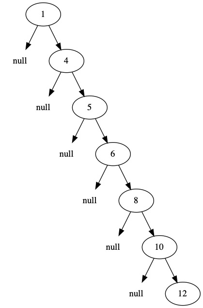
In this case, we have build a linked list. The height is the number of nodes minus one. The worst case height is \(h = n-1\).
The tree we saw earlier was a full balanced tree. Ever position on every level was filled.
First level as 1 node
Second level has 2 nodes
Third level has 4 nodes
Fourth level has 8 nodes
\(k\)-th level has \(2^k\) nodes
The total nodes in the tree is
\( \begin{align} 1+2+4+8+16+\cdots+2^{k} \end{align} \)
This formula should remind you of binary numbers. We are adding powers of two! A tree with \(k\) levels can store as many numbers as a \(k\)-bit binary number. Our tree has \(3\) levels, so it can store \(1+2+4=7\) numbers.
The best case height of a tree is to fill every space. A height must be a whole number, so we need to round down. That means for a tree with \(n\) nodes, we have
\( \begin{align} h = \left\lfloor \log_2(n) \right\rfloor \end{align} \)
The height will fall in a range between these two extreme cases.
\( \begin{align} \left\lfloor \log_2(n) \right\rfloor \le h \le n-1 \end{align} \)
Where will the tree fall in this range? That will depend on the values and the order they are entered. There are a number of modifications to the BST that will force it to always stay balanced. Some examples are AVL Trees, 3-4 Trees, and Red-Black Trees. Each of these data structures tracks the height of the tree and moves values if it becomes to unbalanced. For uniform random values, a standard BST will likely be close to balanced.