Quick Sort
Contents
Quick Sort
The basic idea of Quick Sort is the same as Merge Sort. We want to divide the array in half, then sort the halves. The difference comes in how we divide the array.
The Quick Sort algorithm selects a pivot value. It divides the array into a section that is smaller that the pivot and a section larger than or equal to the pivot. We then recursively sort the two smaller sections.
Partition
To implement Quick Sort, we need to be able to partition the array around a random pivot. If we can’t do this, then it is hopeless to try implementing Quick Sort.
The Partition algorithm takes the start and stop indexes setting the range of elements to partition around. It selects a random element to be the pivot. The random pivot is moved to the last index in the range for partitioning.
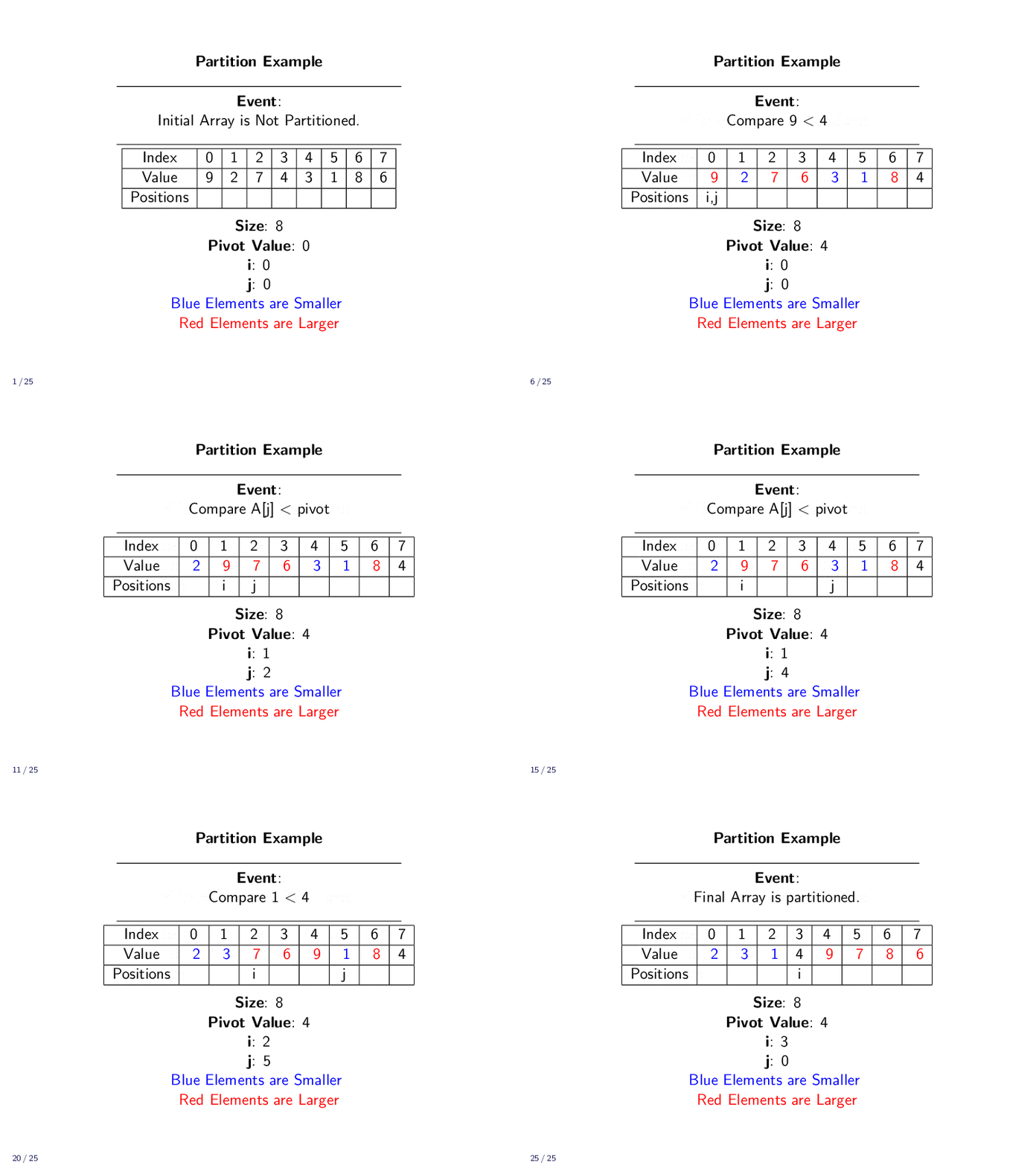
We compare each value to the pivot. If the value is smaller, we put it on the left side of the array. It the value is larger, we put it on the right side of the array. Once we have compared every element to the pivot, we can place the pivot in between the two sections with a final swap.
When the Partition algorithm ends, it returns the index of the pivot. This way we can determine where the smaller and larger elements are.
Partition Example
The following animation shows how the Partition algorithm moves values around in the array.

Partition Implementation
The implementation starts by selecting a random index. To make the implementation easier, we swap this value with the last element in the range. This way we don’t have to try and avoid the pivot during the loop.
The index i tracks the location of the first value larger than the pivot. The index j tracks the value we are comparing to the pivot. When we find a value that it two small, we swap it with the first value larger than the pivot.
Once the loop as ended, all elements are in the right place except the pivot. We swap the pivot with the first larger value. It is now in its final sorted location.
Lastly, we return the index of the pivot element.
Function partition(array pointer A, int start, int stop)
    //Select Random index
    Let randomIndex = randInt(start, stop)
    //Swap with last position
    swap(A, stop, randomIndex)
    //Partition Based on Last Index Pivot
    Let pivot = A[stop]
    Let i = start
    For(j := start; j < stop; j++)
        //Swap a small and large value into place
        If A[j] < pivot then
            swap(A, i, j)
            i = i + 1
        End If
    End For
    //Put the pivot in place
    swap(A, i, stop)
    //Return index of pivot
    Return i
End Function
Partition Analysis
The Partition algorithm only has a single loop. It looks at every element in the range, everything else is constant time. The partition algorithm takes \(O(n)\) to run.
It also uses only a constant amount of memory for the variables and instructions. This means the memory need is \(O(1)\). We only need a pointer to the array, not a copy of the array itself.
Quick Sort Algorithm
Instead of breaking an array perfectly in half, we pick on element at random. We take this element and partition all the items into two smaller sets. Let us call the random pivot value \(p\). The first section of the array is all elements \(x < p\). The second section is \(x \ge p\). The partition sits in between the two sections. It is in its final position since everything to the partition’s left is smaller and all values to its right are larger.
Once we have partitioned around one value, we have to sections of the array. The two sections are not sorted, but we can be sure no elements need to move between sets. All elements are in the correct section. We can call Quick Sort recursively on each section. This will sort the elements correctly.
We keep repeating the recursion until there are no more elements to sort.
Quick Sort Example
The following animation shows how Quick Sort runs over the entire array.
Quick Sort Implementation
The Quick Sort algorithm is implemented recursively. We start with all elements from 0 to size-1. Each recursive call partitions the array around a random value.
The Quick Sort algorithm is called recursively on the two halves of the array based on the partition index.
//QuickSort
Function quicksort(array pointer A, int size)
    qsort(A, 0, size-1)
End Function

Function qsort(array pointer A, int start, int stop)
    If start < stop then
        Let p = partition(A, start, stop)
        qsort(A, start, p-1)
        qsort(A, p+1, stop)
    End If
End Function
Quick Sort Analysis
In the best case, we divide the array exactly in half. We have already seen that the partition is \(O(n)\). This ends up being the exact same runtime as Merge Sort.
\( \begin{align} T(n) =& 2T(n/2) + n \\ =& O(n \log_2(n)) \end{align} \)
What about when we don’t divide exactly? The worse case is a division of 1 element and n-1 elements.
\( \begin{align} T(n) =& T(n-1) + T(1) + n \end{align} \)
We can use expansion to determine the closed form of this worst case. We can also simplify \(T(1)=1\) since sorting 1 element is trivial.
\( \begin{align} T(n) =& T(n-1) + (n+1) & \text{Iteration 1} \\ =& \left( T(n-2) + (n-1)+1 \right) + (n+1) & \text{Expand} \\ =& T(n-2) + n + (n+1) & \text{Iteration 2} \\ =& \left( T(n-3) + (n-2) + 1 \right) + n + (n+1) &\text{Expand} \\ =& T(n-3) + (n-1) + n + (n+1) & \text{Iteration 3} \\ =& \left( T(n-4) + (n-3)+1 \right) + (n-1) + n + (n+1) & \text{Expand} \\ =& T(n-4) + (n-2) + (n-1) + n + (n+1) & \text{Iteration 4} \\ =& T(n-5) + (n-3) + (n-2) + (n-1) + n + (n+1) &\text{Iteration 5} \\ \end{align} \)
You might see a pattern you are familiar with from Insertion Sort begin created. We eventually reach a summation.
\( \begin{align} T(n)=& 1 + 2 + 3 + \cdots + (n-3) + (n-2) + (n-3) + n + n+1 \\ =& \sum_{x=1}^{n+1} x \\ =& \frac{(n+1)^2}{2} + \frac{n+1}{2} \end{align} \)
This is the same pattern we saw during Insertion Sort. The worst case for Quick Sort is it devolved into Insertion Sort and runs in \(O(n^2)\) time.
The memory usage of Quick Sort is linear. In the worst case will complete \(O(n)\) recursive calls. It also needs some constant space for variables and instructions for each of those calls. The overall memory usage is \(O(n)\). In the optimal case, it might only need \(O(\log_2(n))\) recursive calls.
Both probabilistic analysis and practical experimentation have shown that the the worst case is so unlikely that Quick Sort performs at \(O(n \log_2(n))\) in practice. We can again say that for practical purposes the memory usage will also be \(O(\log_2(n))\). The algorithm is easier to implement and makes less copies than Merge Sort, making Quick Sort the most efficient practical algorithm for sorting.

