Depth First Search
Contents
Depth First Search
How do we find out way through a maze?
Look at the maze below. How do you get from the start to the end?

You can probably find a solution very easily. A more interesting problem is to find an algorithm that will solve the problem. This is the question answered by Depth First Search. Given a graph and a starting point, find your way around the graph.
DFS Algorithm
We can imagine Hansel and Gretel leaving a trail of breadcrumbs through the woods. We also need to leave a trail of breadcrumbs as we travel through the graph. This way we don’t get lost and go in a circle.
We create an array to store the breadcrumbs. When we visit a node, we leave a breadcrumb at that node. We travel forward as far as we can without stepping on a node that has breadcrumbs. When we run out of options, we backtrack to an option we skipped earlier.
Function DFS(start node v, graph G, Array breadcrumbs)
    breadcrumbs[v] = True //leave a breadcrumb in this node
    For node in G.adjacentTo(v) do
        If breadcrumbs[w] == False then
            DFS(w,G,breadcrumbs)
        End If
    End For
End Function
We will look through an example to see how the algorithm runs.
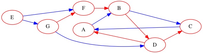
The function takes a starting node. In this case, node A.
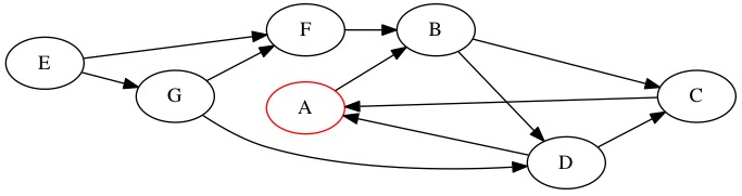
Follow the edge from \(A\) to \(B\).
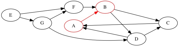
There are two edges from \(B\). We select \(B \rightarrow D\) arbitrarily.
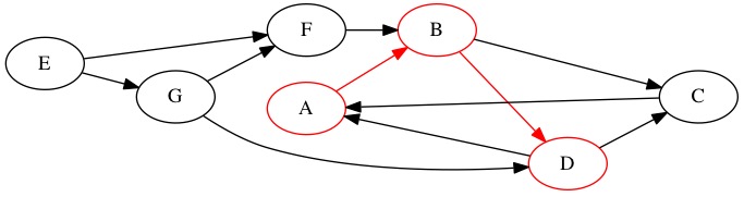
\(D\) has an edge to \(A\) but we have been there. \(D\) has an edge to \(C\).
\(C\) has an edge to \(A\) but we have already been there. We are at a dead end. We need to backtrack. First, check for any additional edges out of \(D\). There is nowhere to else to go from \(D\).
We backtrack to \(B\). There is an edge to \(C\) but we have been there. We Backtrack to \(A\). There are no more edges we can follow. We can never reach \(E, F, G\) starting at \(A\).
We can apply this algorithm to a maze. Imagine each position in the maze is a node. There are edges for paths that player is allowed to move. The goal of the algorithm in this example is to find the exit marked with a E character.
All Paths DFS
In some situations, we might want to run a DFS that reaches every node. This will require starting at more than one position. Some locations cannot reach other locations.
Function dfsAll(Graph G)
    breadcrumbs = newArray()
    For every node $v$ in G do
        DFS(v,G,breadcrumbs)
    End For
End Function
If we are going to do a DFS, just finding the solution is not always the answer. We may want to learn something about the graph as we search. We can then use this knowledge afterwards. Once we do a DFS, we should learn about the graph.
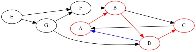
We will revise our concept of breadcrumbs. Previously, we either had a true or false value. All we cared about was not going in circles. In this version, we will track two integers for every node.
foundCounter- Track the order we first discover nodes.finishedCounter- Track the order we close a node. A closed node is one that has no remaining paths. There is nothing left to search from a closed node.
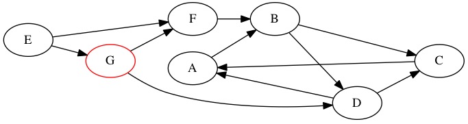
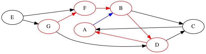
Everything starts at 0 because we have not discovered any nodes yet. We select \(G\) as the starting node. We set \(G\)’s found counter to 1. It is the first thing we have found.
Node |
Found Counter |
Finished Counter |
|---|---|---|
A |
0 |
0 |
B |
0 |
0 |
C |
0 |
0 |
D |
0 |
0 |
E |
0 |
0 |
F |
0 |
0 |
G |
1 |
0 |
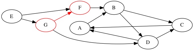
The first node we travel to if \(F\). This is the second node we have found. It gets a 2 in the found counter position.
Node |
Found Counter |
Finished Counter |
|---|---|---|
A |
0 |
0 |
B |
0 |
0 |
C |
0 |
0 |
D |
0 |
0 |
E |
0 |
0 |
F |
2 |
0 |
G |
1 |
0 |
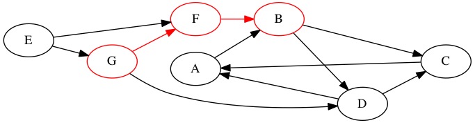
We next discover the node \(B\). It is the third node found.
Node |
Found Counter |
Finished Counter |
|---|---|---|
A |
0 |
0 |
B |
3 |
0 |
C |
0 |
0 |
D |
0 |
0 |
E |
0 |
0 |
F |
2 |
0 |
G |
1 |
0 |
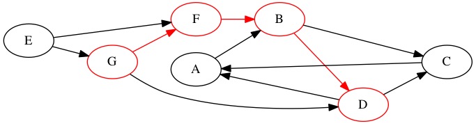
The node \(B\) has multiple outgoing edges. We decide to travel to node \(D\) next.
Node |
Found Counter |
Finished Counter |
|---|---|---|
A |
0 |
0 |
B |
3 |
0 |
C |
0 |
0 |
D |
4 |
0 |
E |
0 |
0 |
F |
2 |
0 |
G |
1 |
0 |
From node \(D\) we continue onward deeper into the graph. We select node $$ as the fifth node found.

Node |
Found Counter |
Finished Counter |
|---|---|---|
A |
5 |
0 |
B |
3 |
0 |
C |
0 |
0 |
D |
4 |
0 |
E |
0 |
0 |
F |
2 |
0 |
G |
1 |
0 |
Here is where things start to get interesting. The node \(A\) has a outgoing edge but it is to a place we have already been! We cannot take this edge. We set \(A\) to have a finished counter. There is no place to go from \(A\) that we have not already been to. The counter has previously set to 5, which means the finished counter is 6 for node \(A\). Having the found and finished counter for node \(A\) be one apart tells us that there was nowhere new to travel to from node \(A\) when we found it.
Node |
Found Counter |
Finished Counter |
|---|---|---|
A |
5 |
6 |
B |
3 |
0 |
C |
0 |
0 |
D |
4 |
0 |
E |
0 |
0 |
F |
2 |
0 |
G |
1 |
0 |
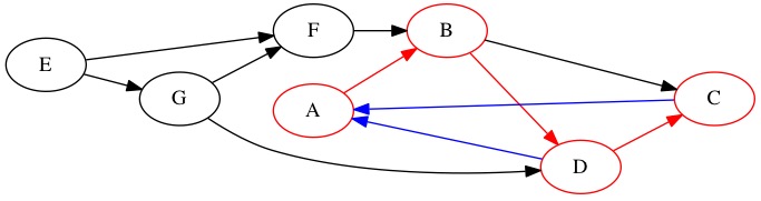
We now backtrack. The node we found before \(A\) was \(D\). It still has potential edges to use. We take the edge to node \(C\).
Node |
Found Counter |
Finished Counter |
|---|---|---|
A |
5 |
6 |
B |
3 |
0 |
C |
7 |
0 |
D |
4 |
0 |
E |
0 |
0 |
F |
2 |
0 |
G |
1 |
0 |
The outgoing edges of node \(C\) travel to places we have already been. It gets a finished counter of 8. Node \(D\) has now run out of edges. It gets a finished counter of 9. We backtrack all the way back to node \(B\) which still has an edge we have never looked at.
Node |
Found Counter |
Finished Counter |
|---|---|---|
A |
5 |
6 |
B |
3 |
0 |
C |
7 |
8 |
D |
4 |
9 |
E |
0 |
0 |
F |
2 |
0 |
G |
1 |
0 |
We learn that node \(B\)’s edge also goes somewhere we have already been. Working backwards we are finished with \(B\) (10) and \(F\) (11). We go all the way back to the starting point \(G\).
Node |
Found Counter |
Finished Counter |
|---|---|---|
A |
5 |
6 |
B |
3 |
10 |
C |
7 |
8 |
D |
4 |
9 |
E |
0 |
0 |
F |
2 |
11 |
G |
1 |
0 |
Although node \(G\) has an unused edge, it takes us somewhere we have been. We close node \(G\) with a 12.

Node |
Found Counter |
Finished Counter |
|---|---|---|
A |
5 |
6 |
B |
3 |
10 |
C |
7 |
8 |
D |
4 |
9 |
E |
0 |
0 |
F |
2 |
11 |
G |
1 |
12 |
There was one node we never visited. Node \(E\) was unreachable. We start the search from this node. It is discovered at counter value 13. It only has edges to places we have been before and gets immediately closed with value 14.
Node |
Found Counter |
Finished Counter |
|---|---|---|
A |
5 |
6 |
B |
3 |
10 |
C |
7 |
8 |
D |
4 |
9 |
E |
13 |
14 |
F |
2 |
11 |
G |
1 |
12 |
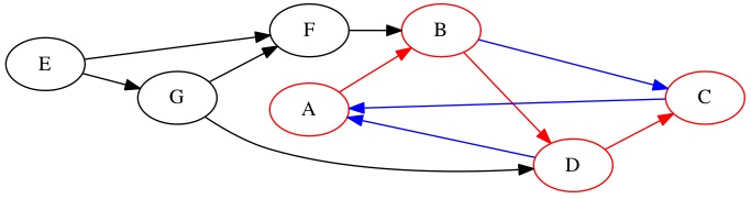
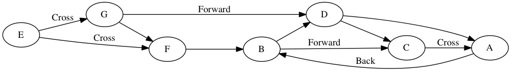
We can learn a lot from the found and finished counters. The graph has four kinds of edges.
Tree Edge - The path we took through the graph made a tree.
Back Edge - These edges take you back to somewhere you have been before creating a cycle.
Forward Edge - These are edges we discovered that are shortcuts forward. They jump you forward on the path the DFS took.
Cross Edge - These edges take you across the graph without going forward/backward.
We can determine what each edge is by looking at the found and finished counter.
The edge from \(F\) to \(B\) is a tree edge. Notice that node \(F\) range is completely within node \(G\). We have \(1 < 2 < 11 < 12\). Additionally, the difference between the found counter is only 1, meaning this was the next thing found.
Node |
Found Counter |
Finished Counter |
|---|---|---|
F |
2 |
11 |
G |
1 |
12 |
Node \(D\) had two children, but we can still see the ranges are all connected by one. Both \(A\) and \(C\) are between \(4\) and \(9\). They cover the entire sequence of numbers in that range.
Node |
Found Counter |
Finished Counter |
|---|---|---|
D |
4 |
9 |
A |
5 |
6 |
C |
7 |
8 |
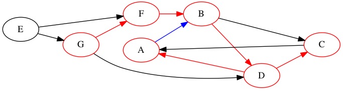
There is an back edge from node \(A\) to \(B\). Node \(A\) has a smaller range \(5-6\) then node \(B\)’s range of \(3-10\). Node B’s range encompasses node \(A\) but the edge goes the opposite direction. This denotes a back edge. It can take you back to somewhere you visited before.
Node |
Found Counter |
Finished Counter |
|---|---|---|
A |
5 |
6 |
B |
3 |
10 |
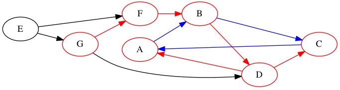
There is a forward edge from node \(G\) to node \(D\). The edge does go from a larger (1-12) range to a smaller (4-9) range. The ranges have gaps between them. This tells us that this edge is a shortcut forward in the graph.
Node |
Found Counter |
Finished Counter |
|---|---|---|
D |
4 |
9 |
G |
1 |
12 |
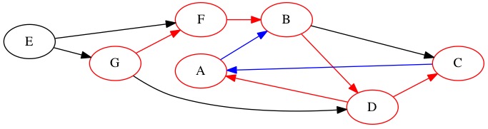
The last type of edge is a cross edge. This connects to ranges that do not overlap. There is a cross edge between node \(C\) and node \(A\). Their ranges do not overlap in any way.
Node |
Found Counter |
Finished Counter |
|---|---|---|
A |
5 |
6 |
C |
7 |
8 |
We can use this information to learn about the graph. If the graph denoted tasks that needed to be completed, a back edge would be a problem. It would be impossible to complete the tasks because they contained a cycle. If it was a maze, the forward edge is a shortcut.
Runtime Analysis
In the worst case, the DFS looks at every edge and every node. The runtime is \(\Theta(V+E)\) or \(\Theta(n+m)\). We use \(V\) or \(n\) for Nodes. We use \(E\) of \(m\) for Edges.
Why have a plus in a Theta Notation? It gives extra information. We cannot predict how many edges there will be relative to nodes. A graph could have 1,000 nodes but only 5 edges. It could also have \(V^2\) edges, with an edge for every possible connection. \(\Theta(V+E)\) is a linear time Graph Algorithm.
DFS can be used to find a path through a graph (or maze). We can find (and remove) cycles in a graph. We can perform a topological sort, which determines order in which tasks must be completed. We can find Strongly Connected Components (SCC). A SCC is a set of vertexes such that every vertex has a path to every other vertex in the set. This means the set must contain a cycle.
A DFS alone tells us about a graph. Taking the results allows us to learn more about the graph. Many algorithms use DFS as a starting point.