Insertion Sort¶

Overview¶

The Bubble Sort algorithms looks at the entire array ever iteration. We always look at every element. What if we only focused on sections of the array?

This is the concept behind Insertion Sort. We start by completely sorting a section of the array. Then we insert more elements into the already sorted area. This will cut down on the amount of times we re-examine each value.

The basic concept goes as follows:

Sort the first two elements
Shift the third element into place
Shift the fourth element into place
Repeatedly shift elements until finished

A single element is sorted by default. There is only way to organize 1 element.

We need two variables to keep track of the current state of the array.

The i variable tracks the first unsorted elements.
The j variable is used to shift the value into position.

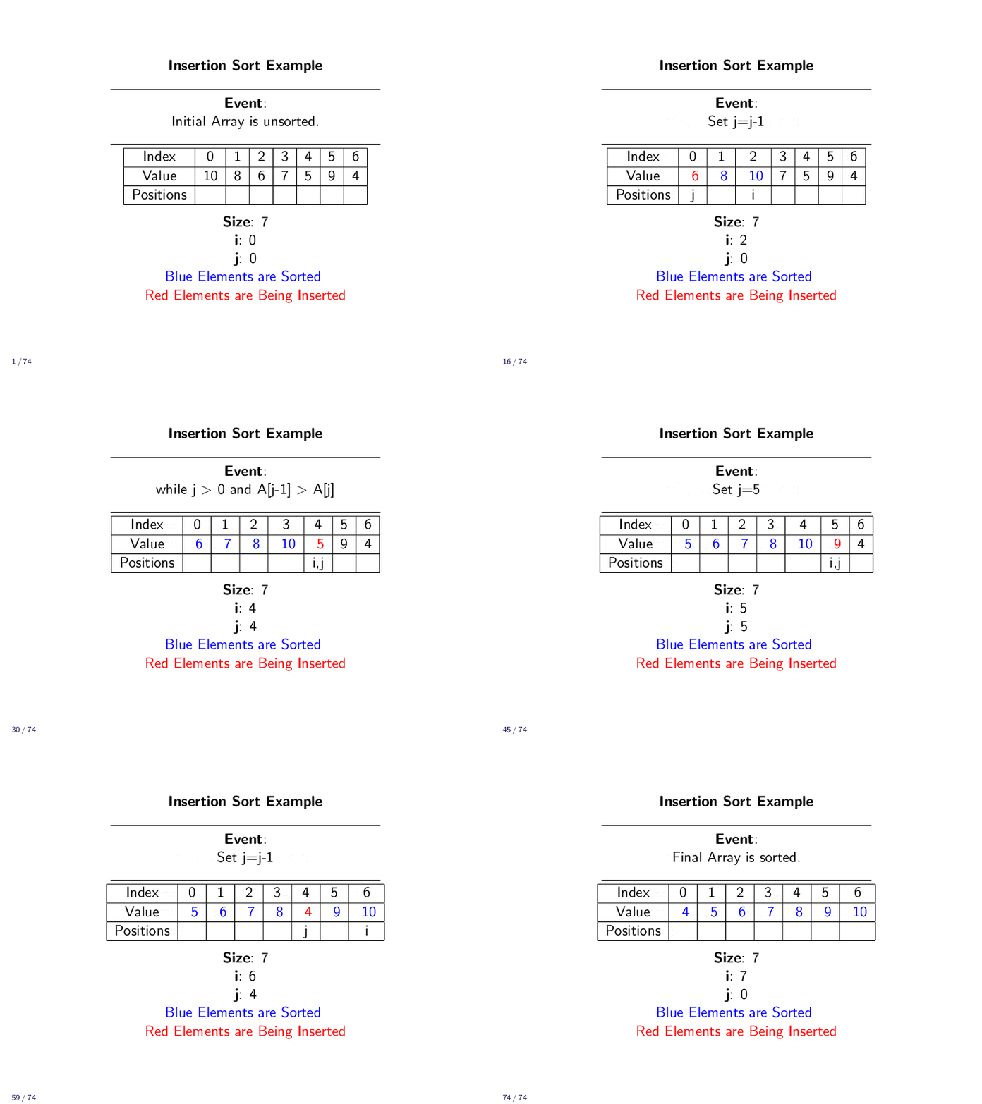
When we start, we set i=1. Element A[0] is trivially sorted. The value at A[1] is the first value we aren’t sure about. We need a loop to shift the value into position.

Unlike Bubble Sort, we have an advantage this time. We know all values from \(0\) to \(i-1\) are sorted. We just need to move A[i] down until a point where it is in the right place.

Example¶

Insertion Sort Example

Implementation¶

The implementation requires nested loops. The outer loop tracks the end of the sorted area of the array. It repeats until there are no unsorted elements remaining.

The inner loop swaps the element at A[j] down until it finds the correct location in the array. At this point, we have 1 additional element sorted correctly.

Function insertion(pointer to array A, integer size)
    Let i = 1 //i tracks first unsorted element
    While i < size do
        //Shift the value A[j] into position
        Let j = i
        While j > 0 and A[j-1] > A[j] do
            Swap values at index j-1 and j in A
            j = j - 1
        End While
        //Update position of first unsorted element
        i = i + 1
    End While
End Function

Analysis¶

How many times do the loops execute?

The outer loop starts at i = 1. It runs until i < size is false. The means the outer loop will execute size-1 times.

What about the inner loop? When i=1, the inner loop runs at most 1 time. When i=2, it does at most 2 iterations. After 2 iterations, you will have moved the element at the end of the array to the front. That is as far as it can go. When i=3, it does at most 3 iterations before the element will be at the front of the array. This continues as i increases. Whatever value i takes, we can do at most i swaps before the element moves to the front of the array. Once the element is at the front of the array, there is nowhere else for it to go.

This describes a summation. In the worst case, we do 1 swap, then 2 swaps, then 3 swaps, etc. In the worst case, every time we compare two elements we need to swap them. If we compare two elements and don’t swap them, the loop will end early.

\( \begin{align} \text{swaps} =& 1 + 2 + 3 + 4 + 5 + \cdots + \left( \text{size}-1 \right) \end{align} \)

We can write this as a summation. Let \(n\) be the size of the array.

\( \begin{align} T(n) =& \sum_{x=1}^{n-1} x \end{align} \)

The following summation is similar and has a well known solution.

\( \begin{align} \sum_{x=0}^{n} x \end{align} \)

We can loop at some of the numbers in the summation to get an idea of what is happening.

\( \begin{align} \sum_{x=0}^{n} x =& 0+ 1 + 2 + 3 + \cdots + (n-3) + (n-2) + (n-1) + n \end{align} \)

What if we pair up the numbers differently?

\( \begin{align} \sum_{x=0}^{n} x =& (0+n)+ (1 + (n-1)) + (2 + (n-2)) + (3 + (n-3)) + \cdots \end{align} \)

Notice that \(0+n=n\) and \(1+(n-1)=n\). Each pair in this ordering adds to up exactly \(n\).

\( \begin{align} 0 + n =& n \\ 1+(n-1) =& n \\ 2+(n-2) =& n \\ 3+(n-3) =& n \\ x+(n-x) =& n \end{align} \)

How many pairs of number will there be? The sum starts at \(0\) and goes to \(n\). That means there are \(n+1\) values. The \(n\) numbers and \(0\). When we pair the numbers up, each pair adds up to \(n\). There are \(\frac{n+1}{2}\) pairs.

If we have \(\frac{n+1}{2}\) pairs and each pair totals to \(n\), then the grand total is \(n * \frac{n+1}{2}\).

\( \begin{align} \sum_{x=0}^{n} x =& n * \frac{n+1}{2} \\ =& \frac{n^2 + n}{2} \\ =& \frac{n^2}{2} + \frac{n}{2} \end{align} \)

We can check this formula for two examples. One even and one odd, just to prove the division works correctly.

\( \begin{align} \sum_{x=0}^{4} x =& 0+1+2+3+4 \\ =& 10 \\ \frac{4^2}{2} + \frac{4}{2} =& \frac{16}{2} + \frac{4}{2} \\ =& 8+2 \\ =& 10 \end{align} \)

\( \begin{align} \sum_{x=0}^{5} x =& 0+1+2+3+4+5 \\ =& 15 \\ \frac{5^2}{2} + \frac{5}{2} =& \frac{25}{2} + \frac{5}{2} \\ =& 12.5 + 2.5\\ =& 15 \end{align} \)

At the end of this chapter, an extended proof of this summation will be give. For now, we will treat it as a fact.

\( \begin{align} \sum_{x=0}^{n} x =& \frac{n^2}{2} + \frac{n}{2} \end{align} \)

This is not exactly the summation we had to Insertion Sort. Ours did not use \(0\) or \(n\).

\( \begin{align} T(n) =& \sum_{x=1}^{n-1} x \end{align} \)

We can relate this to our known summation.

\( \begin{align} T(n) =& \sum_{x=1}^{n-1} x \\ =& \left( \sum_{x=0}^{n} x \right) - 0 - n \\ =& \left( \frac{n^2}{2} + \frac{n}{2} \right) - 0 - n \\ =& \frac{n^2}{2} + \frac{n}{2} - \frac{2n}{n} \\ =& \frac{n^2}{2} - \frac{n}{2} \end{align} \)

In the worst case, Insertion Sort will need to complete \(T(n)=\frac{n^2}{2} - \frac{n}{2}\) swaps.

Everything the algorithm does it determined by how many times it needs to swap. We can get the asymptotic running time.

\( \begin{align} T(n) =& O\left( \frac{n^2}{2} - \frac{n}{2} \right) \\ =& O(n^2) \end{align} \)

Compared to Bubble Sort, we have cut the amount of work in half. It still falls in the same class of algorithms. It is controlled by a quadratic formula.

The runtime of Insertion Sort is \(O(n^2)\).

What about the memory usage? A pointer to the array is passed as input, not the array itself. We just need some variables, but there is a constant amount. We also need constant space for the code itself.

The memory usage of Insertion Sort is \(O(1)\).

Inductive Proof of Summation¶

Let us call the following summation \(S(n)\).

\( \begin{align} S(n) =& \sum_{x=0}^{n} x \end{align} \)

We will prove that

\( \begin{align} S(n) =& \frac{n^2}{2} + \frac{n}{2} \end{align} \)

For all \(n \in \mathbb{N}\).

Base Case¶

We show by example that for small \(n\) the formula is correct.

\( \begin{align} S(0) =& \sum_{x=0}^{0} x =& 0 \\ S(1) =& \sum_{x=0}^{1} x =& 0 + 1 = 1\\ S(2) =& \sum_{x=0}^{2} x =& 0 + 1 + 2 = 3 \\ S(3) =& \sum_{x=0}^{3} x =& 0 + 1 + 2 + 3 = 6\\ S(4) =& \sum_{x=0}^{4} x =& 0 + 1 + 2 + 3 + 4 = 10\\ \end{align} \)

These are the same results as the closed form expression.

\( \begin{align} S(0) =& \frac{0^2}{2} + \frac{0}{2} =& 0 \\ S(1) =& \frac{1^2}{2} + \frac{1}{2} =& \frac{1}{2} + \frac{1}{2} = 1 \\ S(2) =& \frac{2^2}{2} + \frac{2}{2} =& \frac{4}{2} + \frac{2}{2} = 3 \\ S(3) =& \frac{3^2}{2} + \frac{3}{2} =& \frac{9}{2} + \frac{3}{2} = 6 \\ S(4) =& \frac{4^2}{2} + \frac{4}{2} =& \frac{16}{2} + \frac{4}{2} = 10 \\ \end{align} \)

Inductive Case¶

Inductive Hypothesis¶

Let us assume that the equality holds for integer \(k\) in the range \(0 \le k \le n\).

\( \begin{align} S(k) =& \sum_{x=0}^{k} x = \frac{k^2}{2} + \frac{k}{2} \end{align} \)

Inductive Proof¶

We show that if the equality holds for integer \(k\) in the range \(0 \le k \le n\), then it will also hold for \(n+1\).

\( \begin{align} S(n+1) =& \sum_{x=0}^{n+1} x & \text{Evaluate Sum at n+1} \\ =& \left( \sum_{x=0}^{n} x \right) + n+1 & \text{Remove last element from Sum} \\ =& \left( \frac{n^2}{2} + \frac{n}{2} \right) + n+1 & \text{Use Inductive Hypothesis} \\ =& \frac{n^2}{2} + \frac{n}{2} + \frac{2n}{2} + \frac{2}{2} & \text{Find Common Denominator} \\ =& \frac{n^2 + 2n + 1}{n} + \frac{n+1}{2} & \text{Simplify Fractions} \\ =& \frac{ (n+1)^2 }{n} + \frac{n+1}{2} & \text{Simplify Numerator} \end{align} \)

We have show that

\( \begin{align} S(n+1) =& \sum_{x=0}^{n+1} x = \frac{ (n+1)^2 }{n} + \frac{n+1}{2} \end{align} \)

Conclusion¶

We have shown that for all \(k \in \mathbb{N}\)