Breadth First Search
Contents
Breadth First Search
A Depth First Search goes as deep as possible before backtracking and trying other options. What if we want to find all the nodes closest to us first. This problem can be solved by a Breadth First Search (BFS). If all edges have exactly the same weight, a BFS is a shortest path algorithm. It always looks at the closes things first.
The basic idea given below:
Look at everything 1 edge from starting point
Look at everything 2 edges from starting point
Look at everything 3 edges from starting point
etc
We can give high level pseudocode for this concept.
Function BFS(Node start, Graph G)
    Let e=1
    While Graph is not explored do
        Look at all nodes e edges away from start
        e = e + 1
    End While
End Function
This algorithm hides a very important component. It does not explain how we figure out what nodes are \(e\) edges away.
Algorithm Description
To keep track of what nodes to search next, we will use a Queue. As new nodes are found, we will add them to the back of the queue. This will ensure that older nodes are searched before newer nodes.
Function BFS(Node start, Graph G)
    Let Q = makeEmptyQueue()
    Let breadcrumbs = makeEmptyArray(numNodes(G))
    breadcrumbs[start] = True //We have only visited start node
    enqueue(start,Q) //This is the visit node to search
    While not isEmpty(Q) do
        Let x = front(Q)
        dequeue(Q)
        For Node y in adjacentTo(G,x) do
            If breadcrumbs[y]==False then
                breadcrumbs[y]=True
                enqueue(y,Q)
            End If
        End For
    End While
End Function
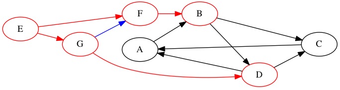
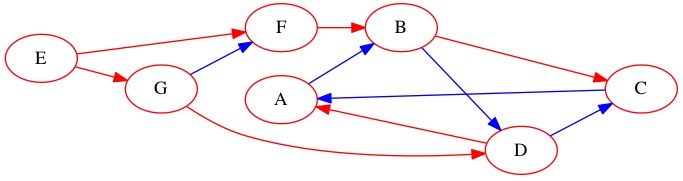
We search the following graph starting at node \(E\).
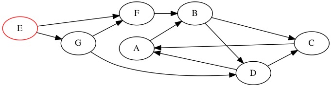
The Queue looks like \(E \rightarrow \text{Null}\). Node \(E\) is the first node discovered, we call this discovery depth zero. It took us zero edges to find node \(E\).
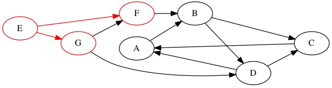
When we dequeue node \(E\) we find it is connected to two adjacent nodes. These are nodes \(F\) and \(G\). They are added to the queue. They have discovery depth one because they are one edge from the start. It doesn’t matter what order we add \(F\) and \(G\) because they are at the same depth.
Queue: \(F \rightarrow G \rightarrow \text{Null}\)
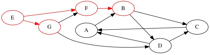
We dequeue node \(F\) and look at it’s adjacent edges. It is connect to \(B\). We add node \(B\) to the queue. Node \(B\) was found at depth two.
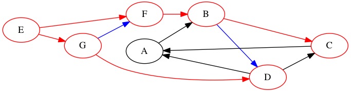
Queue: \(G \rightarrow B \rightarrow \text{Null}\)
We dequeue node \(G\) next. It has one edge to a node we have already seen. We do not add node \(F\) to the queue because we already left a breadcrumb on that node. We do find one new node \(D\). Node \(D\) is at depth 2.
Queue: \(B \rightarrow D \rightarrow \text{Null}\)
Notice that we have looked at all nodes with depth 1. Now we move on to depth 2 nodes. We look at node \(B\) first because it was the first one we found. We learn about new node \(C\). We already knew about \(D\) and it is not added to the queue. Node \(C\) has a depth of 3.
Queue: \(D \rightarrow C \rightarrow \text{Null}\)
Next, we examine node \(D\). We find one edge to a node we have already found, node \(C\). We also find a new node \(A\). Node \(A\) is depth 3 from the start.
Queue: \(C \rightarrow A \rightarrow \text{Null}\)
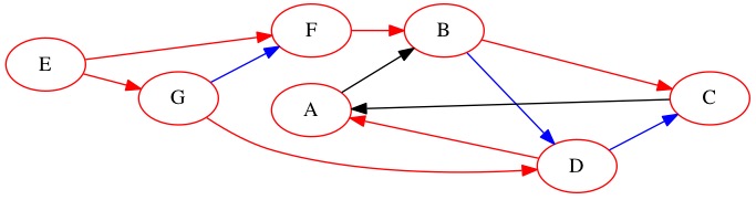
Node \(C\) only has edges to nodes we already new about. We search it, but do not learn anything new.
Queue: \(A \rightarrow \text{Null}\)
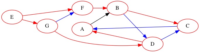
The last node we search is node \(A\). It also has no edges to nodes we didn’t already find.
Queue: \(\text{Null}\)
The queue is now empty. There is nothing more to search. We can exit the algorithm at this point. The depth of each node is listed below.
Depth |
Nodes |
|---|---|
0 |
E |
1 |
G, F |
2 |
B, D |
3 |
C, A |
A BFS searches all the closest places first. This is a classic search pattern in the real world. Imagine you are looking for a lost friend in the woods. You start with places that are closest to where they were seen last. You work out from that point.
The following animation shows a BFS searching for a target in a grid. The algorithm wants to find the character \(T\). It puts an \(X\) in a spot once it has been searched. The algorithm does not move in diagonals for this example.
Applications
The BFS is a shortest path algorithm. If every edge has exactly the same weight, it finds the shortest path to each node. This nodes not scale to arbitrary weights. You could need to add edges to make the BFS function. For example, if an edge has weight 100, you could replace that with 100 edges and find the shortest path. Although this would work, it would be very inefficient compared to Dijkstra. In the animation above, the 2-D grid inherently has equal weights between nodes. This is a great application of BFS.
If you want to know the actual path, you need a predecessor array. When a node is added to the queue, make a note in the predecessor array of who came before it. You can then rebuild the path just like with Dijkstra.
You may also want to know the depth. If this is the case, make a depth array. A node has a depth that is 1 larger than the node it was found by. This is used in web site analysis. Often we want to ask, how many links does it take to get from the main page to a target path. A BFS could answer this question using depths.
If we want to search a website or hard drive for a file, BFS is a great solution. We start at a specific point. We add folders or follow links as needed until we find the file.
We can also use BFS to take an existing graph and find a subgraph with no cycles. We just remove every edge the BFS did not use.
Analysis
The BFS is another linear time graph algorithm. It must look at every node and every edge exactly one time. The queue will at most hold every node in the graph.
The memory usage will be \(O(V)\) for \(V\) nodes. The runtime will be \(O(V + E)\) for \(V\) nodes and \(E\) edges. If a node has many nodes and few edges, the value of \(V\) will overtake \(E\). If the graph is contains every possible edge then \(E=V^2\) and the algorithm will become \(O(V^2)\).