Shortest Paths
Contents
Shortest Paths
Finding the shortest path from point \(A\) to point \(B\) is one of the most straightforward graph problems. It is a problem we encounter every day as humans.
Find the cheapest plane tickets between two cities
Find the shortest path to drive to work
Walk between to classrooms efficiently
Send a message to another computer on the network efficiently
Determining how to get from point \(A\) to point \(B\) often requires finding some intermediate points along the way. We generalize this problem as the Single Source Shortest Path problem. What is the shortest path from node \(A\) to every other node in the graph.
Dijkstra’s Algorithm
We first need to look at how weights are represented to defined what shorted means.
Defining the Shortest Path
Each edge in a graph has a weight. We define this weight as a function of the two edges. The edge from node \(a\) to node \(b\) has the weight \(w(a,b)\).
The weight of a path is the sum of the edges along the path.
Let us assume the graph contains a path \(P=(a,c,b,d)\). This means we can travel from \(a\) to \(d\) by taking edges \(a \rightarrow c\), \(c \rightarrow b\), and \(b \rightarrow d\). The weight of this path is the sum of the edges along the path.
\( \begin{align} w(P) =& \sum_{(u,v) \in P} \left( w(u,v) \right) \\ =& w(a,c) + w(c,b) + w(b,d) \end{align} \)
The shortest path from \(X\) to \(Y\) is the path with the smallest total weight.
There may be multiple shortest paths in a graph. The following image has 2 shortest paths from \(a\) to \(c\). Both have a total weight of 11.
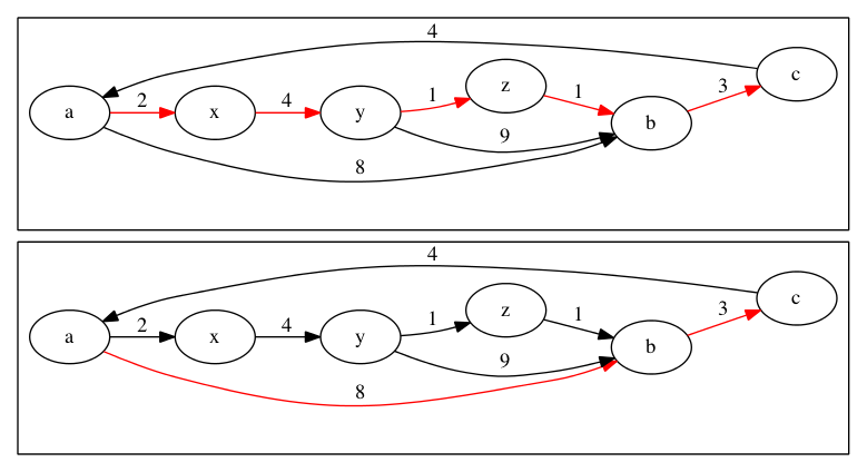
How can we determine the shortest path? If all the edges is the graph are great than zero, we can use the triangle inequality. If edges have positive weights, then adding more edges to a path will always increase the total weight of the path.
The Triangle Inequality allows us to eliminate paths that are not the shortest. We have two paths one from \(s\) to \(u\) and one from \(s\) to \(v\). We also have an edge from \(u\) to \(v\). This means we have two potential paths to \(v\). We should either take the path to \(u\) first and the edge \((u,v)\) or we should take the alternative path to \(v\).
One of the following two formulas must be true.
w(Path(s,u)) + w(u,v) \(<\) w(Path(s,v))
w(Path(s,v)) \(\le\) w(Path(s,u)) + w(u,v)
This can be shown visually as a triangle.

If w(Path(s,u)) + w(u,v) \(<\) w(Path(s,v)) is true then it is better to take the path to u and edge (u,v) instead of our current path. If w(Path(s,v)) \(\le\) w(Path(s,u)) + w(u,v) is true then it is better to use our current path instead of (u,v).
The process of using the triangle inequality to eliminate a path is called relaxation. The function compares two paths and updates an array D with the shortest of the two distances.
Function Relax(Graph G, int u, int v, DistanceArray D)
    If D[v] > D[u] + Weight(G,u,v) then
        D[v] = D[u] + Weight(G, u,v)
    End If
End Function
Dijkstra’s Explained
Dijkstra’s Algorithm uses relaxation to find the shortest path in a graph. It starts by creating a tentative list of distances called D. At the start, we don’t know any real distances. We set the starting node be to \(0\) because we don’t need to travel to it. We set every other node to \(\infty\). Our initial estimate is that is it impossible to get to the nodes.
Next, we initiate a loop. While we have not found all shortest paths, we use relaxation. We select u to be the closest node based on the estimated distances in D. Once we have found a next closest node, we check all the edges of u to see if we can update our D estimates using relaxation.
We need to know what the next closest node is. To find this out, we use a heap! The value at the top of the heap will be the next smallest value.
We will walk through an example to see how this works.
In this graph, we start with the node \(A\). We set it’s distance to 0 and all other nodes to \(\infty\).
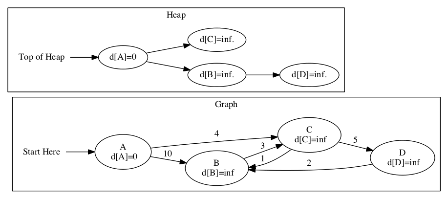
The closest node is node \(A\). We look at the edges of \(A\) and update the distances. We have better estimates for both \(C\) and \(B\). They may not be the best estimate, but they are better. We also update the heap to account for the new distances.
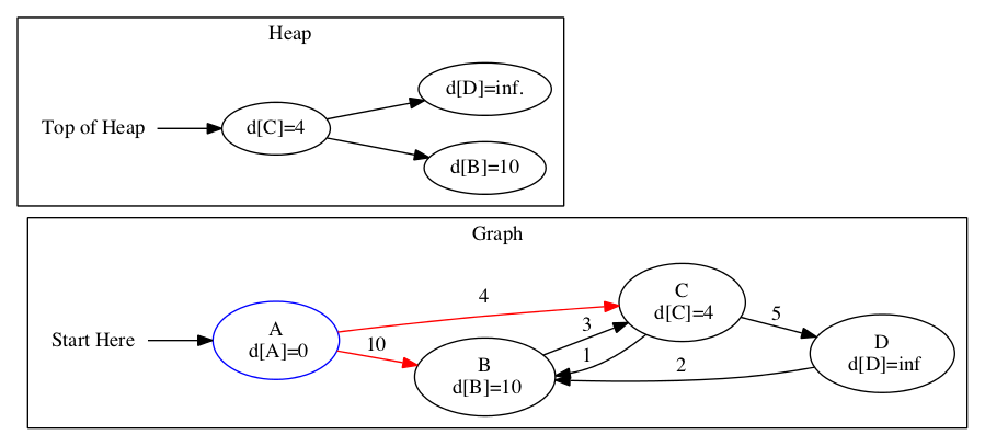
The top of the previous heap was \(C\). We update the distances based on \(C\) and it’s edges. Notice the heap is updated again.
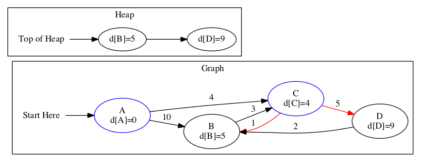
The top of the previous heap was \(B\). We update the heap and distance estimates based on the edges connected to \(B\).
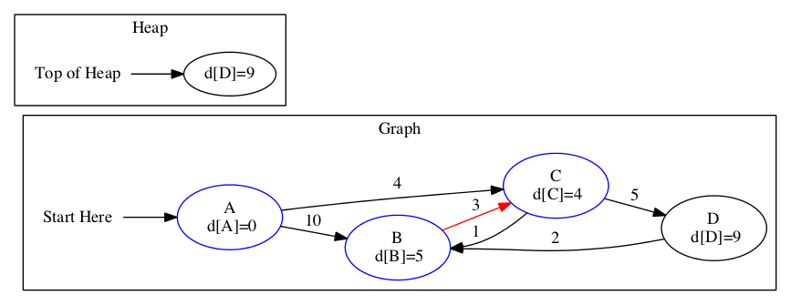
There is only one node left in the heap. We need to update the distance array based on this node. Then we will be done.
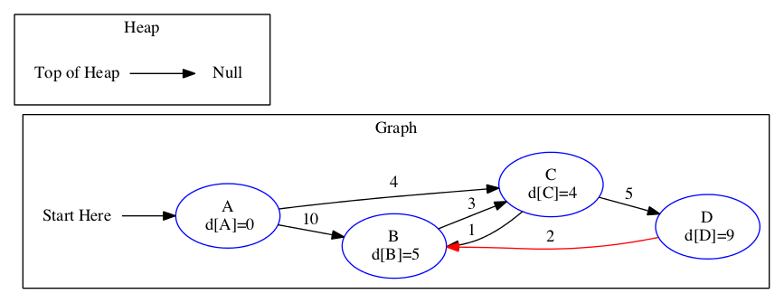
We get the final distances to each node.
Node |
Distance |
|---|---|
A |
0 |
B |
5 |
C |
4 |
D |
9 |
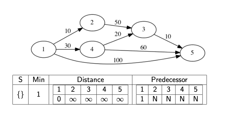
We might actually want to know what the path is, not just it’s distance. In this case, we need to record the predecessor node. This is the node immediately before the current node in the shortest path. If we know the predecessor, we can work backwards to find the full path. We update the predecessor at the same time as we update the distance array.
The following images show a full walkthrough with the distance and predecessor arrays.
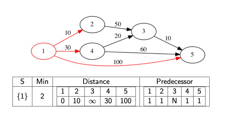
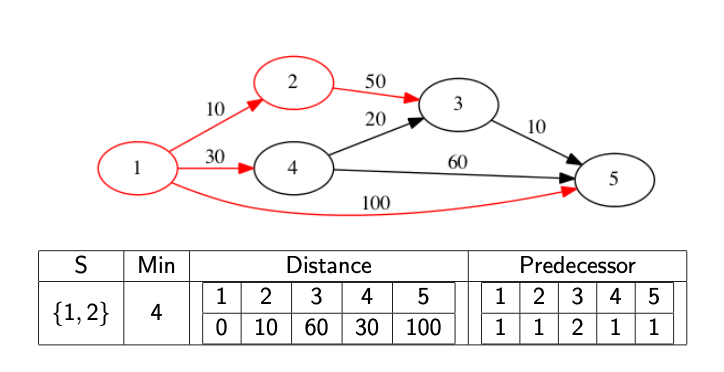
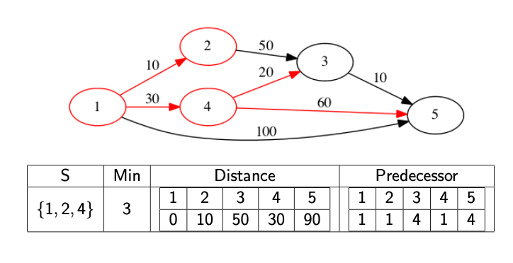
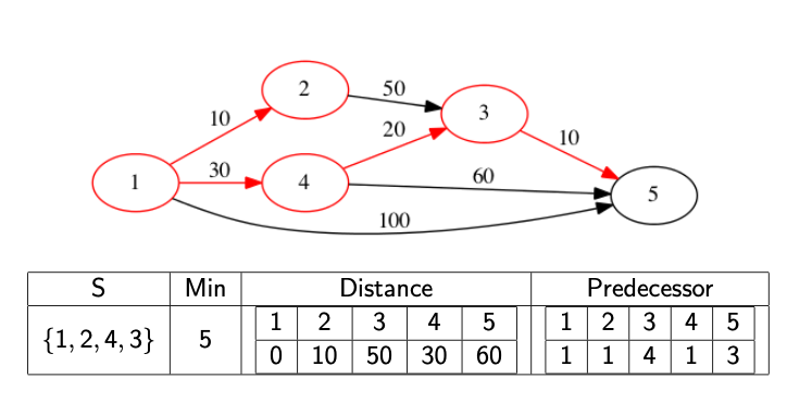
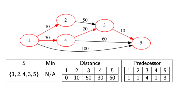
The code below provides a template for finding the distance array.
/*
    Dijkstra's Algorithm
    Compute the Shortest Path to All Nodes
    Does not find the paths in this version
*/

//Dijkstra is an implementation of Dijkstra's Shortest Path Algorithm
Function Dijkstra(Graph G, int startNode)
    //Create the Distance Array
    Let D = newArray(numberNodes(G))
    //Set all values to infinity
    fillArray(D, getInfinity())
    //Set start node to 0
    D[startNode] = 0
    //Create a Priority Queue
    Let PQ = createPriorityQueue(D)
    //We find one path per loop
    While PQ is not empty do
        //Determine the Minimum Node in the Heap
        Let u = minNode(PQ)
        deleteMin(PQ)
        //Determine which nodes are Adjacent
        Let adjList = adjacentTo(G, u)
        //For each Adjacent Node, relax
        For i from 0 until len(adjList) do
            Let v = adjList[i]
            //Relax the Node
            If D[v] > D[u] + weight(G, u, v) then
                D[v] = D[u] + weight(G, u, v)
                //Update the Heap on Changes
                updateNode(PQ, v, D[v])
            End If
        End For
    End While
    Return D
End Function
The runtime of Dijkstra’s algorithm is determined by the number of edges \(E\) and nodes \(V\). Creating the initial priority queue takes \(O( V \log_2 V)\). The heap could have multiple elements, but it is still controlled by \(V\). The maximum numbers of edges is \(E=V^2\). By the logarithmic rules, we have \(\log_2 (V^2) = 2 \log_2(V) = O(\log_{2}V)\). We need to call extract-min on the heap \(V\) times. Each time takes \(O(\log_{2} V)\). This totals \(O(V \log_{2} V)\). We also need to update the heap. The heap might need to get updated for every single edge in the graph. Updating the heap takes a total of \(O(E \log_{2} V)\). This gives us a final running time of \(O( V \log_{2} V + E \log_{2} V)\).
If all edges have weight \(w(u,v) > 0\) then the node with the current shortest path must be correct. Adding any additional edges to that path will make a longer path. That means it cannot be the shortest. Cycles would also increase the path’s total and would never be part of the shortest path. If \(w(u,v)=0\) then the distance will not change when the edge is added.
Dijkstra’s algorithm will not work if \(w(u,v) < 0\). In these cases, increasing the number of edges in the path will actually lead to a shorter path.

If the graph contains negative weight cycles, then no shortest path exists. The shortest path would be an infinity loop around the negative weight cycle in this case.
In the following graph, we should take the path (2,3,4,2) infinitely.

Bellman-Ford Algorithm
The Bellman-Ford algorithm can handle negative weight cycles. It takes longer than Dijkstra. There are situations where we need to deal with negative weight cycles. One example is currency arbitrage.
The number in this example are from [Pai, September 2019].
A currency exchange is a graph. I have 100.00 USD. I convert USD to PLN (Polish Zloty) at rate 3.93. Now, I have 393.00 Polish Zloty. Next, I covert PLN to EUR (Euros) at rate 0.23. I now have 90.39 EUR. Finally, I convert EUR to USD at 0.90. I end up with 81.35 USD.
We ended up with less then we started with. There will be some neutral paths in the graph where we end up with the same amount we started with. There will be some paths where we lose money. The interesting paths are the ones where we make money. In practice, there are fees related to exchanging money. This is only useful if we can find the paths we make money on quickly and transfer large amounts of money quickly.
Call the rate from \(A\) to \(B\) be called \(w_{A,B}\). An exchange is profitable if
\( \begin{align} w_{A,B}*w_{B,C}*w_{C,D}*\cdots*w_{X,A} > 1 \end{align} \)
If we take the \(\log\) of both sides, then formula becomes an addition.
\( \begin{align} \log(w_{A,B})+\log(w_{B,C})+\log(w_{C,D})+\cdots+\log(w_{X,A}) > 0 \end{align} \)
If we multiply by -1, it becomes a subtraction problem.
\( \begin{align} -\log(w_{A,B})-\log(w_{B,C})-\log(w_{C,D})-\cdots-\log(w_{X,A}) < 0 \end{align} \)
If there exists a negative weight cycle in this format, then there is a profitable exchange in the original graph.
The currency exchange rates are still a graph.
From/To |
PLN |
EUR |
USD |
RUB |
INR |
MXN |
|---|---|---|---|---|---|---|
PLN |
1.00 |
0.23 |
0.25 |
16.43 |
18.21 |
4.94 |
EUR |
4.34 |
1.00 |
1.11 |
71.40 |
79.09 |
21.44 |
USD |
3.93 |
0.90 |
1.00 |
64.52 |
71.48 |
19.37 |
RUB |
0.06 |
0.01 |
0.01 |
1.00 |
1.11 |
0.30 |
INR |
0.06 |
0.01 |
0.01 |
0.90 |
1.00 |
0.27 |
MXN |
0.20 |
0.05 |
0.05 |
3.33 |
3.69 |
1.00 |
After \(-\log(x)\) applied, we have a new matrix.
From/To |
PLN |
EUR |
USD |
RUB |
INR |
MXN |
|---|---|---|---|---|---|---|
PLN |
-0.00 |
1.47 |
1.39 |
-2.80 |
-2.90 |
-1.60 |
EUR |
-1.47 |
-0.00 |
-0.10 |
-4.27 |
-4.37 |
-3.07 |
USD |
-1.37 |
0.11 |
-0.00 |
-4.17 |
-4.27 |
-2.96 |
RUB |
2.80 |
4.27 |
4.20 |
-0.00 |
-0.10 |
1.20 |
INR |
2.90 |
4.34 |
4.27 |
0.11 |
-0.00 |
1.31 |
MXN |
1.61 |
3.06 |
2.96 |
-1.20 |
-1.31 |
-0.00 |
Bellman-Ford is slower then Dijkstra but it can deal with Negative Cycles. It is similar to Dijkstra, but we relax all edges in all combinations. This way we can catch negative cycles. If we relax everything and then relax one more time, only negative weight cycles will change.
The algorithm is show blew.
BellmanFord(Adj Matrix W, Source Node s)
    n = Number of Nodes
    D=Array with n Infinity Values
    P=Array with n Negative One Values
    D[s]=0
    //Find all the shortest paths
    For int i=0; i < n-1; i++ do
        For int u=0; u < n; u++ do
            For int v=0; u < n; v++ do
                If D[u] + W[u][v] < D[v] then
                    D[v]=D[u]+W[u][v]
                    P[v]=u
                End If
            End For
        End For
    End For
    //Find Negative Cycles
    Cycles = A Linked List
    For int u=0; u < n; u++ do
        For int v=0; v < n; v++ do
            If(D[u]+W[u][v] < D[v] then
                //Negative Cycle!
                Append v, u to a linked list cycle
                While P[u]  is not in the cycle do
                    Append P[u] to cycle
                    u=P[u]
                End While
                append P[u] to cycle
                Reverse cycle
                Add entire cycle to Cycles
            End If
        End For
    End For
    //Return the cycles
    Return Cycles
}
We find paths that contain a negative weight cycle.
Cycle Found:
If you had 100.0 RUB
Convert to 111.00 INR
Convert to 6.11 PLN
Convert to 100.31 RUB
The cycle might appear inside the full path.
Cycle Found:
If you had 100.0 USD
Convert to 1937.00 MXN
Convert to 100.72 USD
Convert to 6498.71 RUB
Convert to 7213.57 INR
Convert to 93.78 EUR
Convert to 406.99 PLN
Depth First Search could find the cycle in the path.
Cycle Found:
If you had 100.0 USD
Convert to 1937.00 MXN
Convert to 100.72 USD
Convert to 395.85 PLN
The running Bellman-Ford is \(\Theta(V^3)\) where \(V\) is the number of nodes. The space needed is \(\Theta(V^2)\).
