Algorithm Analysis
Contents
Algorithm Analysis
It is great to be able to say that an algorithm takes exactly \(5n+7\) move operations to print a string with \(n\) characters. This kind of granularity is almost never available or useful. When working in high level languages, we give up this kind of granular analysis. Instead, we are forced to approximate the number of operations.
In practice, we will find that as long as this analysis is done accurately, it provides more useful and general results. We can analyze an algorithm not just a specific implementation.
We need a formal method to compare to algorithms. Something inspired by counting assembly operations, but that can be applied to general algorithms.
Big Oh
The foundation of this method is based on growth rates. We don’t want to pick specific cases and compute their values. We want to talk about how the algorithm scales as the input gets larger. This allows us to compare the performance trend.
It also helps to focus on the worst case situation. As computer scientists, we always need to be prepared for the worst case to happen. It might not always happen, but we need to be prepared. Imagine you went to a party and the host told you “The best case is the muffins are blueberry and the worst case is they are poisoned.” You shouldn’t make a decision based exclusively on the best case.
The most common method of analysis is Big Oh (also called Big-O). The Big Oh is used to provide an approximate upper bound on the runtime of an algorithm.
Big Oh Definition
\(T(n)\) is \(O(f(n))\) if and only if there exists constants \(c>0\) and \(n_0 \ge 0\) such that \(0 \le T(n) \le cf(n)\) for all \(n \ge n_0\).
This definition is very dense and mathematical. Let’s unpack the concepts within.
What are we measuring? We traditionally call this function \(T(n)\), but what does that mean. We need to measure something. We are abstractly trying to estimate the time the code will take, but that is not a practical measure. A faster processor can do more work in less time, but it still does the same amount of operations.
We want to measure work instead of time. This might be directly related to the operations, but it might be more abstract. We could say work is the number of MOV commands the processor does. It may be the case that we want to estimate work as number of network calls or exponents computed. Whatever makes the most sense for the algorithm in question.
The function \(T(n)\) tells us how much work is done for input \(n\). The variable \(n\) is a measure of the size of the input. This could be the size of an array, or the number we are computing with. It could also be more abstract, like the number of frames in a movie. The key is the \(n\) is some measure of the size of the input. Bigger inputs tend to make problems harder to solve.
Think about the problem of printing a string, we could say
\(n\) is the number of letters we need to print
\(T(n)\) is the number of operations needed to print the string
We can estimate our print as \(T(n) = O(n)\). We now get to use the rest of our definition to explain what this means.
exists constants \(c>0\) and \(n_0 \ge 0\) such that \(T(n) \le cf(n)\) for all \(n \ge n_0\)
We have defined \(f(n)=n\) by stating \(T(n) = O(n)\). The value of \(f(n)\) is whatever in in the parenthesis of \(O(\cdots)\). Using this definition gives us the following
\( \begin{align} T(n) \le& cn \end{align} \)
This is telling us the number of yes/no question is always less than \(cn\) for numbers larger then \(n_0\). This is still an abstract definition, let us pick some specific numbers to make it more relatable.
Imagine we did a detailed analysis of the assembly code for a print function and determined it required exactly \(T(n)=7n+7\) operations. Let’s compare this to the function \(9n\).
\(n\) |
\(T(n)\) |
\(9n\) |
|---|---|---|
1 |
14 |
9 |
2 |
21 |
18 |
3 |
28 |
27 |
4 |
35 |
36 |
5 |
42 |
45 |
6 |
49 |
54 |
7 |
56 |
63 |
8 |
63 |
72 |
9 |
70 |
81 |
10 |
77 |
90 |
11 |
84 |
99 |
12 |
91 |
108 |
13 |
98 |
117 |
14 |
105 |
126 |
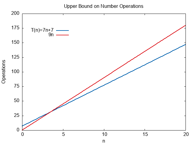
Notice that for all numbers \(n \ge 4\) we see that \(T(n) < 9n\). We can use this to define an upper bound on the value of \(T(n)\). We can start \(T(n) < 9n\) for all values \(n \ge 4\).
In terms of Big-Oh, we call the constant multiplier \(c\) and the starting value \(n_0\).
\( \begin{align} c =& 9 \\ n_0 =& 4 \end{align} \)
We can plot the two expressions. Notice that after \(n=4\) the function \(9n\) always stays above \(7n+7\). It provides an upper bound estimate on the number of operations.
For our specific problem, we are saying
The number of operations will be less than or equal to the nine times the size of the array for any array with 4 or more elements.
Formally, we just write \(T(n)=O(n)\). This says the grow rate of our function is linear, it is bounded by \(c*n\) for some value of \(c\). When comparing algorithms the value of \(c\) only matters if the \(O(f(n))\) values are the same.
The specific value of \(c\) being 9 or 7 or 20 isn’t going to contribute much compared to the exponent of \(n\). An algorithm that is \(O(n^2)\) is growing much faster than one that is \(O(n)\). The constant will become more important when comparing two \(O(n)\) algorithms.
Note
Algorithm Speed and growth rate can cause some confusing terminology.
Growth Rate: How fast the size of the output grows with relation to the size of the input.
Algorithm Runtime: How long the algorithm will take to run.
A fast growth rate means a slow algorithm. The number of operations increases rapidly, causing a slow algorithm.
A slow growth rate means a fast algorithm. The number of operations increases slowly, causing the runtime to stay lower.
Big Oh Basics
The formal definition of Big Oh leads to many applications and concepts. We will break down a few of the most common ones needed in this section. Think of these are the Rules of Thumb for Big Oh analysis.
Tight vs Loose Bounds
The Big Oh can be used to define tight or loose bounds. Since it is based on \(T(n) \le cf(n)\).
Let us assume we have a program that does \(T(n)=5n-7\) MOV operations.
All the following would be true.
\( \begin{align} T(n) =& O(n) \\ T(n) =& O(n^2) \\ T(n) =& O(n^{10}) \end{align} \)
It is technically true that \(T(n) = O(n^{10})\) because we can write
\( \begin{align} 5n-7 \le 5n^{10} \text{ for all n greater than equal to 1} \end{align} \)
We would call this a loose bound. It is correct, but it is terrible estimate.
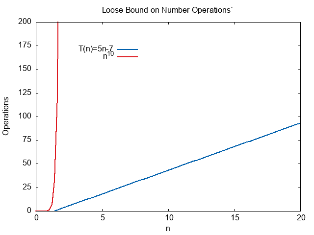
On the other hand, \(T(n)=O(n)\) is a tight bound.
\( \begin{align} 5n-7 \le 5n \text{ for all n greater than equal to 1} \end{align} \)
is as close as we can get with integers. Since the formula is \(cn\) in the Big Oh definition, we can never account for the constant \(-7\).
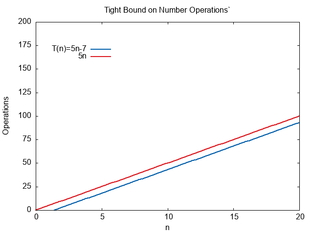
Unless explicitly noted, Big Oh notation is always assumed to mean tight bounds. Although loose bounds are technically correct, they are not very useful. In the corporate and academic world, tight bounds are used almost exclusively. We want the tightest possible bound, then our analysis will be as accurate as possible.
Polynomials
A polynomial is any expression of the form
\( \begin{align} f(x) = a_b x^{b} + a_{b-1} x^{b-1} + \cdots + a_1 x + a_0 \end{align} \)
Any polynomial expression is Big Oh of its largest exponent.
\( \begin{align} f(x) = O(x^{b}) \end{align} \)
For example,
\( \begin{align} g(x) =& 5x^2+9x+7 \\ g(x) =& O(x^2) \end{align} \)
Logarithms
The logarithm is the inverse of the exponent.
\( \begin{align} \log_{a}(a^b) =& b \end{align} \)
A \(\log\) grows faster than a constant, but slower than a polynomial.
The base of a logarithm doesn’t matter for Big Oh notation. All logarithms are multiples of the natural logarithm.
\( \begin{align*} \log_a(b) =& \frac{\ln(b)}{\ln(a)} \end{align*} \)
That means we can pick any base \(a\) and state
\( \begin{align} \log_a(b) =& O(\log_2(b))) \end{align} \)
Computer Scientists use \(\log_2(x)\) so often it is shorted to \(\lg(x)\).
Common Running Times
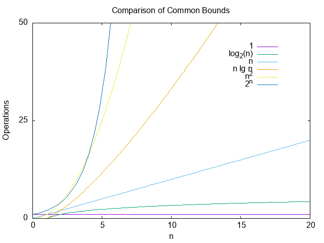
The following are common running times sorted from fastest to slowest.
Big Oh |
Comments |
|---|---|
\(O(1)\) |
Constant Time. The algorithm always does the same amount of work |
\(O(\log_2(n))\) |
Logarithmic Time |
\(O(n)\) |
Linear Time |
\(O(n \log_2(n))\) |
Log-Linear Time |
\(O(n^2)\) |
Quadratic Time |
\(O(2^n)\) |
Exponential Time |
The following plots shows how the different common times compare.
