.md .pdf

Contents

Huffman Encoding

N-Arity Trees

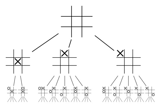
A tree can have any number of children. One time trees with larger numbers of children are needed is in game analysis. We can build a tree showing all the different moves a player can make in a game. The following tree shows possible moves in a Tic-Tac-Toe game.

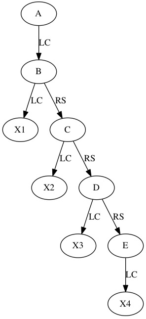
We can represent trees even if we don’t know how many children each one will have. We basically make two linked lists. The first linked list is the Leftmost Child Pointer. It allows us to move down one level in the tree. It points to the first child. The second pointer is the Right Sibling Pointer. It allows you to move across the children at the same level.

• Leftmost Child Pointer - Node’s Child on far left

• Right Sibling Pointer - Next Node to the Right in the tree

Now, we can build trees with any number of children

In this graph, Node 5 has 3 children! This is fine because we can just follow the linked list chain as far as we need to travel.

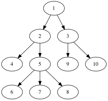
To represent this, we just store two pointers in each node. This is a useful table. Even with only a binary tree, you can describe all the nodes using a table like this. the Table shows each node in the above image and its two pointers.

Node	Leftmost Child	Right Sibling
node1	LMC=node2	RS=none
node2	LMC=node4	RS=node3
node3	LMC=node9	RS=none
node4	LMC=none	RS=node5
node5	LMC=node6	RS=none
node6	LMC=none	RS=node7
node7	LMC=none	RS=node8
node8	LMC=none	RS=none
node9	LMC=none	RS=node10
node10	LMC=none	RS=none

In many cases, pointer are easier to work with. There are some situations where this table would be an advantage.

• What if we have limited memory?

• What if we have a fixed size tree to import?

We can also store this table describing the three into an array of structures. We make an array of triples and it stores everything that needs to be known about the data. This is especially useful for saving the tree to a file and loading it again later.

The above tree can be stored in a 3 by 10 array

Index	LMC	Value	RS
0	1	“1”	-1
1	3	“2”	2
2	5	“3”	-1
3	-1	“4”	4
4	7	“5”	-1
5	-1	“9”	6
6	-1	“10”	-1
7	-1	“6”	8
8	-1	“7”	9
9	-1	“8”	-1

One advantage of storing trees in an array is we can use the same array to store multiple trees. Add one more column parent, a root is a node with parent=-1. A group of trees is called a forest. Forests can be used to compress data.

Huffman Codes

Huffman Codes use trees to compress data. it is often used as a part of compression techniques. Some examples that use Huffman as a part of their encoding technique are given below.

• PKZIP

• MP3

• JPEG

• BZIP

• PNG

Huffman codes are one of the foundations of modern compression.

To get the basic idea with can image a simple text file. Huffman is easiest to visualize on text files because we are all used to working with letters. It is harder to image pixels or frequencies.

1. Break the item up into blocks

2. Compute probability each word in used throughout file

3. Generate Huffman Codes

4. Output symbol table and encoded file

In practice, we could use any binary blocks of data. As long as we can break the file up into blocks that can be organized, it will work. Letters are just fantastic blocks of data to compress text with.

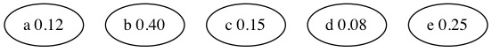
Assume we already computed these probabilities for an imaginary text file.

Letter	Probability
a	12%
b	40%
c	15%
d	8%
e	25%

We start with a tree for every letter with its probability. We have a forest of trees.

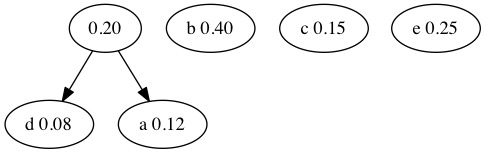
We select the trees with the lowest probabilities and combine them. The new node has a probability that is the sum of its two children. We select the nodes with probability 0.12 and 0.08 nodes combine. This makes a new tree with a total probability of 0.20. To find the two smallest nodes, we can use a heap!

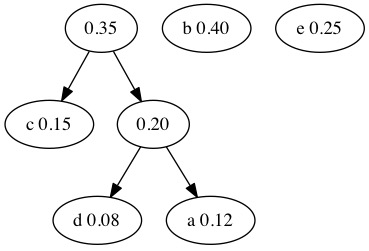
Next we search the forest for the next two smallest nodes. The 0.20 and 0.15 nodes combine. We traditionally put the smaller value on the left and the larger on the right.

The process continues and we combine the 0.35 and 0.25 nodes.

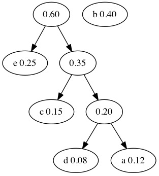
We only have two nodes left. We combine the 0.60 and 0.40 nodes. When only one tree remains in the forest, we have a tree that can be used for compression.

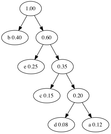
We now generate binary codes to use for each letter. We walk the tree and label the edges.

• Put a Zero on left child

• Put a One on right child

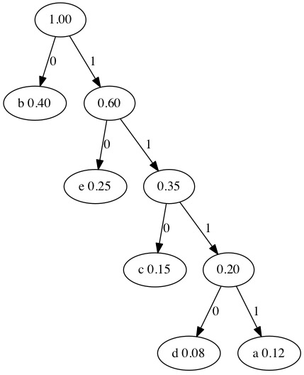
We can walk the three one more time to encode the letters. The path to a letter is the compressed binary representation of that letter.

Letter	Code
a	1111
b	0
c	110
d	1110
e	10

In binary. each character is 8 bits. If we have 1,000,000 8-bit characters that must take up 0.9 megabytes. If the file contains repeated characters, we can save space. Compressed we have 0.25 megabytes for the same file.

Letter	Percentage	Code	Occurrences	Size
a	12%	1111	120,000	480,000 bits
b	40%	0	400,000	400,000 bits
c	15%	110	150,000	450,000 bits
d	8%	1110	80,000	320,000 bits
e	25%	10	250,000	500,000 bits

We compress the file. Characters that do not appear are not given a binary representation at all. Characters that appear frequently have the shortest binary representations. This means we save the most space on the characters that appear the most frequently.

A Second Example

It is not always the case that the tree will be lopsided. It is determined by the probabilities. When many letters have similar probabilities of appearing in the data, the tree will be more balanced. This second example generates a more balanced tree.

Letter	Probability
a	14%
b	8%
c	13%
d	24%
e	7%
f	34%

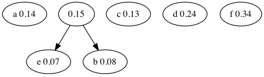
We start with a forest of trees with one node each.

We combine the two smallest probabilities. This combines \(0.08+0.07=0.15\).

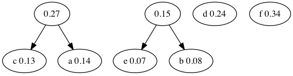
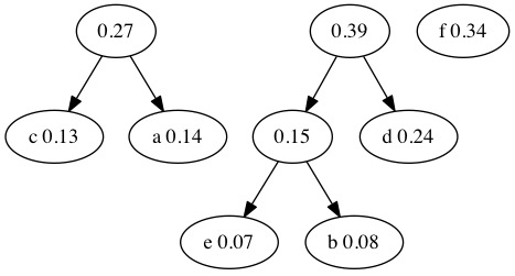
Combine the next two smallest probabilities. Notice that the tree we created in the previous step did not have the smallest probability. We now have two trees. The nodes that merge are \(0.14+0.13=0.27\).

Combine the next two smallest probabilities. This time we return to the tree from a previous step. We combine \(0.15+0.24=0.39\).

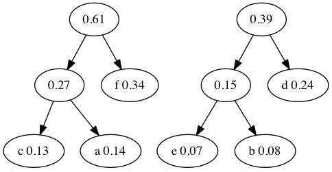
When we combine the two smallest probabilities, we return to the probability 27 tree from earlier. Merge \(0.27+0.34=0.61\).

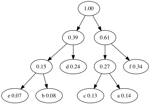
We only have two tree left in our forest. We combine \(0.61+0.39=1.00\). The tree is finished because 100% of the characters are now accounted for.

To generate the Huffman Codes, we put a 0 on left branches and a 1 on right branches.

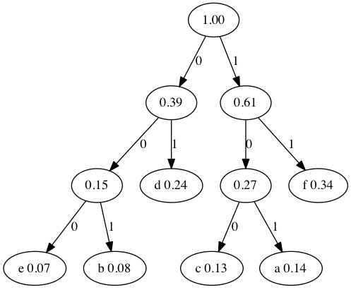
We can determine how much this compresses our tree. Again, a classical binary representation of characters requires 8 bits per letter. If we had 2,000,000 8-bit characters with the probabilities listed above it would require 2 megabytes. Since this data doesn’t use many letters we compress it down to 0.605 megabytes without losing any data.

Letter	Percentage	Code	Occurrences	Size
a	14%	101	280,000	840,000 bits
b	8%	001	160,000	480,000 bits
c	13%	100	260,000	780,000 bits
d	24%	01	480,000	960,000 bits
e	7%	000	140,000	420,000 bits
f	34%	11	680,000	1,360,000 bits

Huffman Encoding is a lossless compression scheme. It finds the optimal binary representations of each letter and compresses the data. The key is that is takes advantage of the data it is compressing to build the tree. It is an distinct tree for the file being compressed. If you were to try and generate a Huffman Encoding for all valid ASCII characters with equal weights you would just recreate ASCII. It is only because not every letter is used at the same frequency in every file that this method works well.

Decompression

All the information needed to decode is stored in the tree. Lets look at a short string in binary from the larger file. We will decompress 010110111000100 using the tree below.

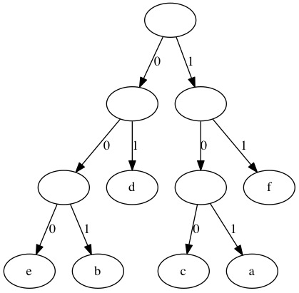
We use the bits to find a path through the tree from the root to a leaf. The first two bits lead to a lead in the tree.

010110111000100

Following the edges 0 and 1 takes us to a leaf. This decodes as d and we go back to the root of the tree for the next bit.

d0110111000100

Following the edges 0 and 1 takes us to a leaf. This decodes as d and we go back to the root of the tree.

dd10111000100

We need to read three bits to get to the next leaf. This decodes as a.

dda11000100

We only need two bits for the next path to read a leaf. the value 11 decodes as f.

ddaf000100

The next three bits 000 decode as e.

ddafe100

The final three bits 100 decode as c.

ddafec

We have recovered the original string. The information we need to decode is stored in the tree. Compared to the file size, the tree doesn’t use much memory.

We could store this tree using 2*(11 short (16-bit)) + 11 char (8-bit) = 440 bits extra data. In reality, more bits would probably be needed to explain the table start and end points as well as other extra info like file created date. Regardless, for a large file this extra data will be tiny by comparison.

The decompression tree can be stored as in a table as shown below.

Index	LMC	Value	RS
0	1	None	-1
1	2	None	6
2	3	None	5
3	-1	e	4
4	-1	b	-1
5	-1	d	-1
6	7	None	-1
7	9	None	8
8	-1	f	-1
9	-1	c	10
10	-1	a	-1

Algorithm Overview

This code provides an outline for creating the Huffman codes for a file. It relies heavily on concepts from data structures like the Heap and Binary Search Tree that we have already seen. Without all those tools, this algorithm would appear far more complicated.

    float* count = countLetters(filename);
    //Find Grand Total of letters
    int total=0;
    //This examples assumes only char 0-128 are used
    for(int i=0; i < 128; i++){
        total=total+count[i];
    }
    //Make a Heap with max 128 spaces
    Heap* H = makeHeap(128);
    //Add all the nodes
    for(int i=0; i < 128; i++){
        //Only add letters that appear at least once
        if(count[i] > 0){
            hNode* n = newHuffNode(i,count[i]);
            insert(n,H);
        }
    }
    //Select Two Smallest nodes
    //Until Forest is merged
    while(size(H)!=1){
        hNode* A = min(H);
        deletemin(H);
        hNode* B = min(H);
        deletemin(H);
        A = merge(A,B);
        insert(A,H);
    }
    //Display the Final Answer
    hNode* final = min(H);
    deletemin(H);
    //Make the table
    CodeBank* CB = generateCodes(final);
    printCodeBank(CB);

previous

Heaps

next

Introduction to Graphs