Asymptotic Analysis
Contents
Asymptotic Analysis
Asymptotic Comparisons
What happens when to a function when it’s input gets very big? What happens when it gets infinitely large?
These are the foundational questions of asymptotic analysis. We don’t want to talk about any specific input to the function. We want to describe what happens as the inputs get larger.
Let’s take a simple function \(f(x)=5x^2 + 3x - 3\).
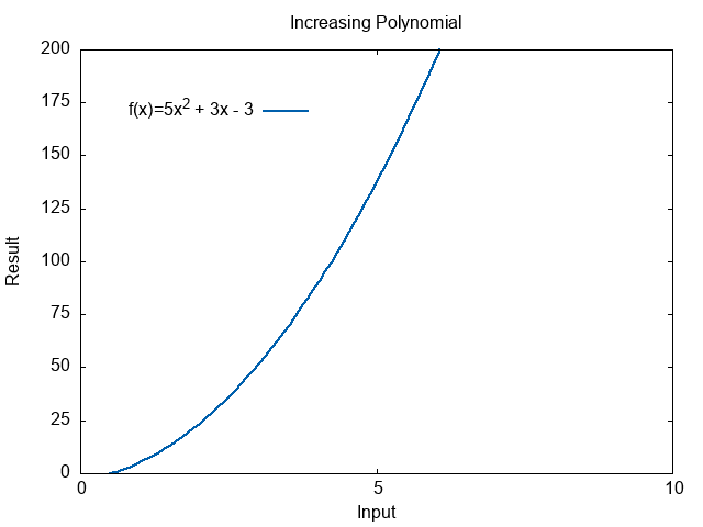
What happens when this function gets larger?
\( \begin{align} f(100) =& 50297 \\ f(1000) =& 5002997 \\ f(10000) =& 500029997 \end{align} \)
The first thing we should notice is as the input gets larger, the result also gets larger. The function is increasing.
How much do the different parts of the expression contribute to the result as the input increases? First, let us look at the contribution to the function of the \(-3\) at the end. At \(f(100)\) the answer is 50,297. If we didn’t subtract 3 at the end, the result would be 50,300. The difference between the values is only \(0.006\%\) of the correct answer. If we look at \(f(10000)\) the subtract by three changes the answer by \(0.000001\%\).
We will look at the ratio between two expressions to compare how they change. If we compute \(\frac{7}{25}=0.28\), we would say that \(7\) is \(28\%\) of \(25\). If you got a discount of \(28\%\) on a item costing \(25\) dollars, you would get \(7\) dollars off.
We can look at the ratio \(\frac{f(x)}{5x^2 + 3x}\). This will tell us how close we are to the correct answer.
\(x\) |
\(f(x)\) |
\(5x^2+3x\) |
Ratio |
|---|---|---|---|
100 |
50297 |
50300 |
0.9999403578528827 |
1000 |
5002997 |
5003000 |
0.9999994003597841 |
10000 |
500029997 |
500030000 |
0.9999999940003600 |
100000 |
50000299997 |
50000300000 |
0.9999999999400003 |
1000000 |
5000002999997 |
5000003000000 |
0.9999999999994000 |
The ratio gets closer and closer to \(1.0\) as the size increases. It will never reach it exactly, but the difference caused by subtracting three becomes ever more meaningless.
As the size of \(x\) increases in \(f(x)\), it is fair to say the \(-3\) doesn’t contribute much. We can claim that as \(x\) increases the answer is very close to \(5x^2+3x\). They are not exactly equal, but for large numbers the difference is tiny. We use the \(\sim\) symbol to show that the expressions are asymptotically equivalent.
\( \begin{align} (5x^2 + 3x - 3) \sim & (5x^2 + 3x) \\ f(x) \sim 5x^2 + 3x \end{align} \)
We have determined that the \(-3\) does not have a significant impact on the result as the input gets very large. What about the \(3x\)? We can look at another ratio. The ratios are easiest for humans to read when they are \(\text{Smaller} / \text{Larger}\). This time we will put \(f(x)\) on the top because it will be larger. This won’t matter for formal analysis, but it makes the table easier to visualize. We compute the ratio \(\frac{(5x^2 + 3x - 3)}{5x^3}\).
\(x\) |
\(f(x)\) |
\(5x^2\) |
Ratio |
|---|---|---|---|
100 |
50297 |
50000 |
0.9940950752529972 |
1000 |
5002997 |
5000000 |
0.9994009590651364 |
10000 |
500029997 |
500000000 |
0.9999400095990642 |
100000 |
50000299997 |
50000000000 |
0.9999940000959990 |
1000000 |
5000002999997 |
5000000000000 |
0.9999994000009600 |
10000000 |
500000029999997 |
500000000000000 |
0.9999999400000096 |
When we get to \(f(1000000)\) the solution to \(5x^2\) is \(99.9999\%\) of the exact answer. We can again say the result is asymptotically equivalent.
\( \begin{align} f(x) \sim 5x^2 \end{align} \)
We are saying that as \(x\) gets very large, the value of \(f(x)\) is really just the value of \(5x^2\). It is not exactly the same, but it is very close. The larger \(x\) gets, the closer the two get to each other.
What we say that \(5x^2\) is a exceptionally good approximation for \(f(x)\) when \(x\) is very large.
Limits
The formal method for asking “what happens for very large numbers” is the limit. We ask “what is the limit of the function as it’s input approaches infinity.” Since infinity is the largest number there is, approaching infinity means as number get really large heading towards infinity.
Let us return to our function \(f(x)=5x^2 + 3x - 3\). What value does this function approach as \(x\) approaches infinity?
\( \begin{align} \lim_{x \rightarrow \infty} f(x) = \infty \end{align} \)
The answer to our question is infinity. The larger \(x\) gets, the larger \(f(x)\) gets in response. Since they both keep going up, larger inputs cause larger outputs. If we imagine that we keep giving the function bigger inputs forever, it will give us larger outputs forever. It’s outputs approach infinity as the inputs approaches infinity.
Note
In Computer Science, we look at inputs greater than or equal to 0. We also only look at inputs that are increasing. What would it means to have an array with -12 letters in it?
In pure mathematics, we have to worry about negative, imaginary, or irrational values. They won’t appear in Algorithm Analysis.
There are only four primary results of the limit function.
Functions that increase forever towards infinity.
Functions that decrease forever towards negative infinity.
Functions that increase, but never pass an upper max.
Functions that decrease, but never pass a lower min.
We already saw an example of the first case with \(f(x)=5x^2 + 3x - 3\). This function goes up forever.
Decrease Towards Negative Infinity
What if we looked at \(g(x)=-3x\)? This function decreases as \(x\) increases. It goes down forever.
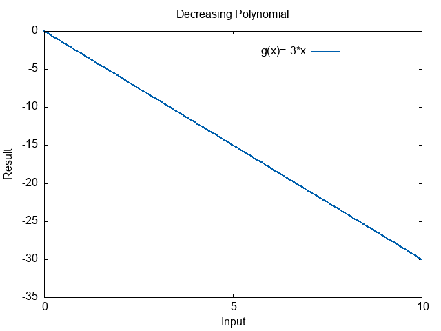
We would say this function has a limit of negative infinity. As the input increases, it goes down forever.
\( \begin{align} \lim_{x \rightarrow \infty}(-3x) = -\infty \end{align} \)
Decrease Towards Constant
Some functions head up or down, but have an boundary they will never cross. Look at the plot of the function \(h(x)= \frac{5}{x}\).
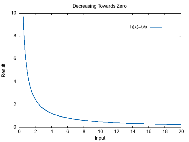
This function goes down, but it will never become negative. No matter how big \(x\) is, \(\frac{5}{x}\) can never be negative. That can only happen if \(x < 0\), not when \(x\) is increasing. This function goes towards 0 as the input increases. It heads in the direction of 0, but never reaches it or passes it.
\( \begin{align} \lim_{x \rightarrow \infty}\left(\frac{5}{x} \right) = 0 \end{align} \)
Increasing Towards Constant
What if we return to our ratio from the previous section? What happens to
\( r(x) = \frac{5x^2}{(5x^2 + 3x - 3)} \)
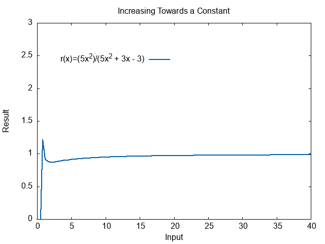
This function increases, it has a peak at the very start. The it slowly creeps up again. It will never increase past 1. The numerator and denominator will never be perfectly equal, but they keep getting closer. As this function approaches infinity, the result approaches 1. It heads towards 1, but never reaches it. Notice that when \(x\) is very small the function does actually go above 1. We are looking at the pattern as the input goes towards infinity. Irregularities at small numbers don’t matter.
\( \begin{align} \lim_{x \rightarrow \infty}\left(\frac{5x^2}{(5x^2 + 3x - 3)} \right) = 1 \end{align} \)
Common Limit Rules
There are a few common rules for dealing with limits.
Let \(a(x)\) and \(b(x)\) be two functions. Additionally, let us assume there is a constant \(c\) that is great than or equal to one.
When determining the limit of an addition, it is the same as adding the limit of the components.
\( \begin{align} \lim_{x \rightarrow \infty} \left( a(x) + b(x) \right) = \lim_{x \rightarrow \infty} \left( a(x) \right) + \lim_{x \rightarrow \infty} \left( b(x)\right) \end{align} \)
The limit of a product is the product of the limits.
\( \begin{align} \lim_{x \rightarrow \infty} \left( a(x) * b(x) \right) = \lim_{x \rightarrow \infty} \left( a(x) \right) * \lim_{x \rightarrow \infty} \left( b(x)\right) \end{align} \)
The limit of a constant is the constant.
\( \begin{align} \lim_{x \rightarrow \infty} \left( c \right) = c \end{align} \)
Using the pervious two rules together, we can pull a constant out of a limit.
\( \begin{align} \lim_{x \rightarrow \infty} \left( c * a(x) \right) = c * \lim_{x \rightarrow \infty} \left( a(x)\right) \end{align} \)
The limit of \(x\) to any constant is infinity.
\( \begin{align} \lim_{x \rightarrow \infty} \left( x^c \right) = \infty \end{align} \)
The limit of a fraction where the denominator is increasing faster than the numerator is zero.
\( \begin{align} \lim_{x \rightarrow \infty} \left( \frac{1}{x^c} \right) = 0 \end{align} \)
The limit of a fraction where the numerator is increasing faster than the denominator is infinity.
\( \begin{align} \lim_{x \rightarrow \infty} \left( \frac{x^2}{5x} \right) = \infty \end{align} \)
Ratio Limits
In Algorithm Analysis, we will always be comparing two functions. Neither of the functions will be decreasing. Any useful algorithm will increase in time as the input increases, or at least stay the same. Algorithms don’t tend to go faster the more data you give them.
Let us assume we have two algorithm’s whose growth rates increase over time.
\( \begin{align} f(n) =& 5n^2 + 3n + 2 \\ g(n) =& 7n+1 \end{align} \)
The number of operations completed by both algorithms increases towards infinity as the size of the inputs increase.
\( \begin{align} \lim_{n \rightarrow \infty} f(n) =& \infty \\ \lim_{n \rightarrow \infty} g(n) =& \infty \end{align} \)
The question here we need to ask is not which function goes to infinity, the question is “which function goes to infinity faster?”. The function that heads towards infinity faster, will have more operations and therefore be a slower algorithm.
We ask what the limit of the ratio is.
\( \begin{align} \lim_{n \rightarrow \infty} \frac{f(n)}{g(n)} =& ? \end{align} \)
We can plot the ratio to get a feel for what is happening.
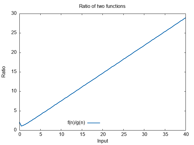
The ratio looks like it heads towards infinity.
We can also formally analyze the limit itself.
\( \begin{align} \lim_{n \rightarrow \infty} \frac{f(n)}{g(n)} =& \lim_{n \rightarrow \infty} \left( \frac{5n^2 + 3n + 2}{ 7n+1} \right) \\ =& \lim_{n \rightarrow \infty} \left( \frac{5n^2}{7n+1} + \frac{3n}{7n+1} + \frac{2}{ 7n+1} \right) \\ =& \lim_{n \rightarrow \infty} \left( \frac{5n^2}{7n+1} \right) + \lim_{n \rightarrow \infty} \left( \frac{3n}{7n+1} \right) + \lim_{n \rightarrow \infty} \left( \frac{2}{ 7n+1} \right) \\ =& \infty + \frac{3}{7} + 0 \\ =& \infty \end{align} \)
The limit goes towards infinity. That tells us the following things.
\(f(n)\) has a higher growth rate than \(g(n)\)
\(g(n)\) has a slower growth rate than \(f(n)\)
\(f(n)\) is a slower algorithm than \(g(n)\)
\(g(n)\) is a faster algorithm than \(f(n)\)
Analysis of Algorithms Definitions
The limit of a ratio between two function forms the basis for the defintions in the Analysis of Algorithms.
There are three primary outcomes when comparing two functions.
\( \begin{align} \lim_{n \rightarrow \infty} \left( \frac{f(n)}{g(n)} \right) =& \infty \\ \lim_{n \rightarrow \infty} \left( \frac{f(n)}{g(n)} \right) =& \text{constant} \\ \lim_{n \rightarrow \infty} \left( \frac{f(n)}{g(n)} \right) =& 0 \end{align} \)
These three different cases are used to define the different symbols in Algorithm Analysis.
Little Oh
The Little Oh is used to define a loose upper bound.
Little Oh Definition
\(T(n)\) is \(o(f(n))\) if and only if for every possible constant \(c>0\) there exists an \(n_0 \ge 0\) such that for all \(n \ge n_0\) we have \(0 \le T(n) \le cf(n)\)
The loose upper bound is defined using limits as
\( \begin{align} \lim_{n \rightarrow \infty} \left( \frac{f(n)}{T(n)} \right) =& \infty \\ \end{align} \)
The function \(f(n)\) goes towards infinity so much faster than \(T(n)\) that the ratio goes towards infinity.
For example, we could take
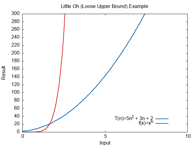
\( T(n) = 5n^2 + 3n + 2 \)
This is loosely upper bounded by \(n^6\).
\( T(n) = o(n^6) \)
The following plot shows how much faster \(n^6\) heads towards infinity.
The limit of the ratio heads towards infinity was well.
\( \begin{align} \lim_{n \rightarrow \infty} \left( \frac{f(n)}{T(n)} \right) =& \lim_{n \rightarrow \infty} \left( \frac{n^6}{5n^2 + 3n + 2} \right) \\ =& \lim_{n \rightarrow \infty} \left( \frac{n^6}{5n^2} \right) \\ =& \lim_{n \rightarrow \infty} \left( \frac{n^4}{5} \right) \\ =& \infty \end{align} \)
Our statement \(T(n) = o(n^6)\) conveys that \(cn^6\) will be an upper bound on \(T(n)\) regradless of what constant you pick for \(c\). The function just grows to much faster. It will always end up as an upper bound.
Little Omega
The Little Omega symbol is used to define a loose lower bound. This is a drastic underestimation of the value.
Little Omega Definition
\(T(n)\) is \(\omega(f(n))\) if and only if for every possible constant \(c>0\) there exists an \(n_0 \ge 0\) such that for all \(n \ge n_0\) we have \(0 \le cf(n) \le T(n)\)
The loose lower bound is defined using limits as
\( \begin{align} \lim_{n \rightarrow \infty} \left( \frac{f(n)}{T(n)} \right) =& 0 \\ \end{align} \)
The function \(f(n)\) goes towards infinity so much slower than \(T(n)\) that the ratio goes towards 0.
For example, we could take
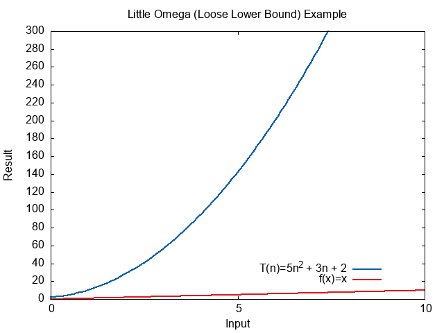
\( T(n) = 5n^2 + 3n + 2 \)
This is loosely lower bounded by \(n\).
\( T(n) = \omega(n) \)
The following plot shows how much slower \(n\) heads towards infinity.
The limit of the ratio heads towards zero, because the denominator is larger than the numerator.
\( \begin{align} \lim_{n \rightarrow \infty} \left( \frac{f(n)}{T(n)} \right) =& \lim_{n \rightarrow \infty} \left( \frac{n}{5n^2 + 3n + 2} \right) \\ =& \lim_{n \rightarrow \infty} \left( \frac{n}{5n^2} \right) \\ =& \lim_{n \rightarrow \infty} \left( \frac{1}{5n} \right) \\ =& 0 \end{align} \)
Our statement \(T(n) = \omega(n)\) conveys that \(cn\) will be a lower bound on \(T(n)\) regradless of what constant you pick for \(c\). The function just grows to slow. It will always end up below \(T(n)\).
Theta
The Theta symbol is used to define a tight bound. This is the most accurate estimate we can make.
Theta Definition
\(T(n)\) is \(\Theta(f(n))\) if and only if there exist two constants \(c_1>0\) and \(c_2 > 0\) and there exists an \(n_0 \ge 0\) such that for all \(n \ge n_0\) we have \(c_1 f(n) \le T(n) \le c_2 f(n)\)
The tight bound is defined using limits as
\( \begin{align} \lim_{n \rightarrow \infty} \left( \frac{f(n)}{T(n)} \right) =& \text{constant} \\ \end{align} \)
The function \(f(n)\) and \(T(n)\) go towards infinity at such a close rate, there is just a constant value as the ratio.
For example, we could take
\( T(n) = 5n^2 + 3n + 2 \)
This is tightly bounded by \(n^2\).
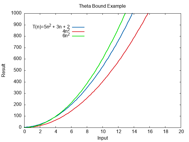
\( T(n) = \Theta(n^2) \)
We need to pick our constants for the upper and lower bound.
\( 4n^2 \le 5n^2 + 3n + 2 \le 6n^2 \)
The following plot shows how \(T(n)\) always stays between the two expressions.
The limit of the ratio heads towards a constant, because the denominator and numerator grow at the same rate.
\( \begin{align} \lim_{n \rightarrow \infty} \left( \frac{f(n)}{T(n)} \right) =& \lim_{n \rightarrow \infty} \left( \frac{n^2}{5n^2 + 3n + 2} \right) \\ =& \lim_{n \rightarrow \infty} \left( \frac{n^2}{5n^2} \right) \\ =& \lim_{n \rightarrow \infty} \left( \frac{1}{5} \right) \\ =& \frac{1}{5} \end{align} \)
Our statement \(T(n) = \Theta(n^2)\) conveys that \(cn^2\) will be an extremely tight estimate for \(T(n)\). The function just grows at exactly the same rate as \(T(n)\).
Big Oh
The Big Oh Symbol defines an upper bound, the bound can be loose or tight. The formal definition is given below.
Big Oh Definition
\(T(n)\) is \(O(f(n))\) if and only if there exists constants \(c>0\) and \(n_0 \ge 0\) such that \(0 \le T(n) \le cf(n)\) for all \(n \ge n_0\).
In terms of limits, this symbol is best defined in terms of two other symbols.
Big Oh Definition
\(T(n)\) is \(O(f(n))\) if and only if \(T(n)\) is \(o(f(n))\) or \(T(n)\) is \(\Theta(f(n))\).
In terms of limits, this means the limit approaches either a constant or infinity. If the limit approaches infinity, we would define it as a loose bound. If the limit approaches a constant, we would define it as a tight bound. In either case, it would be a Big Oh bound.
Big Omega
The Big Omega Symbol defines a lower bound, the bound can be loose or tight. This is Big Oh’s lower bound opposite. The formal definition is given below.
Big Omega Definition
\(T(n)\) is \(\Omega(f(n))\) if and only if there exists constants \(c>0\) and \(n_0 \ge 0\) such that \(0 \le cf(n) \le T(n)\) for all \(n \ge n_0\).
In terms of limits, this symbol is best defined in terms of two other symbols.
Big Omega Definition
\(T(n)\) is \(O(f(n))\) if and only if \(T(n)\) is \(\omega(f(n))\) or \(T(n)\) is \(\Theta(f(n))\).
In terms of limits, this means the limit approaches either a constant or 0. If the limit approaches 0, we would define it as a loose bound. If the limit approaches a constant, we would define it as a tight bound. In either case, it would be a Big Omega bound.