Fast Modular Power¶

The modular exponentiation of a number is the result of computing an exponent followed by getting the remainder from division. This is a common requirement in cryptography problems. The modular exponentiation is useful before the size of the result is bounded. It will never produce a number larger than the modulus.

We treat the modular exponent as a three input function.

\( \begin{align} \text{modPow}(a,b,n) = (a^b) \mod n \end{align} \)

We can compute the modular exponent of \(5^2\) under modulus \(9\).

\( \begin{align} \text{modPow}(5,2,9) =& (5^2) \mod 9 \\ =& 25 \mod 9 \\ =& 7 \end{align} \)

Naive Approach¶

The most obvious solution is just to compute the exponent and then take the remainder. This is very inefficient usage of memory. Let’s look at one example.

\( \begin{align} \text{modPower}(5,28,9) =& (5^{28}) \mod 9 \\ =& 37252902984619140625 \mod 9 \\ =& 4 \end{align} \)

The number 37252902984619140625 requires 66 bits to store. Even with a 64 bit processor, we would overflow with this number! The inputs \(5\), \(28\), and \(9\) could all fit on a 8-bit processor. The result \(4\) could also fit in only 8 bits. Along the way, we would need to store a 66 bit number somehow.

We can keep this number smaller by computing the remainder at multiple steps. We can use the following relationship.

\( \begin{align} (a^2) \mod n =& \left( (a \mod n) * (a \mod n) \right) \mod n \end{align} \)

We can look at this expression with an example first.

\(\begin{align} (28^2) \mod 9 =& 784 \mod 9 \\ =& 1 \end{align} \)

We can compute the same thing using the other side of the relationship.

\( \begin{align} (28 \mod 9) * (28 \mod 9) \mod 9 =& (1 * 1) \mod 9 \\ =& 1 \end{align} \)

Notice that the second expression computes much smaller number in the intermediate step. Remember that the modulo is based on the quotient and remainder. For a specific modulus \(n\) we can write a number \(a\) in terms of the quotient \(q\) and remainder \(r\).

\( \begin{align} a=& q * n + r \end{align} \)

We can compute the square of this number.

\(\begin{align} a^2 =& (qn+r)(qn+r) = q^2*n^2 + 2qnr + r^2 \\ \end{align} \)

What happens when we divide \(a^2\) by the modulus \(n\)?

\( \begin{align} \frac{a^2}{n} =& \frac{q^2*n^2 + 2qnr + r^2}{n} \\ =& \frac{q^2*n^2}{n} + \frac{2qnr}{n} + \frac{r^2}{n} \\ =& q^2*n + 2qr + \frac{r^2}{n} \end{align} \)

The first two terms divide evenly by \(n\). Only the last term \(\frac{r^2}{n}\) does not. Any remainder of the entire expression for \(a^2\) must come from this component. We can compute the remainders and square them without worrying about the rest of the expression.

We can turn this into an algorithm. We just repeatedly compute products and take remainders.

//Compute Mod Exponent using a loop
Function modPower(integer a, integer b, integer n)
    Let temp = 1
    While b > 0 do
        temp = (temp * a) % n
        b = b - 1
    End While
    Return temp
End Function

We could use this method to compute \(\text{modPower}(5,28,9)\) an 8-bit processor! The values will never get to big to overflow memory!

This keeps our memory usage down. We just need to have enough space for the initial inputs. We will never need to store a number larger than \(n^2\) after that point. The largest remainder is \((n-1)\) and we might have to square it before we can take the remainder again.

The next question is how much work is the processor doing. We need to do \(b\) multiplications, subtractions, and remainder calculations. This would end up being a linear time algorithm. It would take \(O(n)\) operations. Assuming that we fix the size of our numbers, say we are working with integers, then memory is constant \(O(1)\).

We can decrease the number of mathematical operations needed.

Fast Mod Power¶

There are some key properties to realize to save work in this problem. The first is that squaring numbers is faster than just multiplying by the base. For example, if we want to compute \(5^6\) we could do it two ways.

First, we compute all the multiplications by \(5\).

\(\begin{align} 5^6 =& 5*(5^5) \\ =& 5*(5*(5^4)) \\ =& 5*(5*(5*(5^3))) \\ =& 5*(5*(5*(5*(5^2)))) \\ =& 5*(5*(5*(5*(5*(5^1))))) \\ =& 5*(5*(5*(5*(5*(5*5^0))))) \\ =& 5*(5*(5*(5*(5*(5*1))))) \\ =& 5*(5*(5*(5*(5*5)))) &\text{Multiply 1: 5 times 1}\\ =& 5*(5*(5*(5*25))) &\text{Multiply 2: 5 times 5}\\ =& 5*(5*(5*125)) &\text{Multiply 3: 5 times 25}\\ =& 5*(5*625) &\text{Multiply 4: 5 times 125}\\ =& 5*3125 &\text{Multiply 5: 5 times 625}\\ =& 15625 &\text{Multiply 6: 5 times 3125} \end{align} \)

We had to compute 6 multiplications to generate this number. We can get to larger number faster by repeated squaring. Once we compute \(5*5=25\), we can reuse 25 to compute \(25*25=625=5^4\). We can use the following relationship on exponents to get to larger powers faster.

\( \begin{align} a^b * a^b =& a^{2b} \end{align} \)

If we want to compute \(5^6\) we can do it easier if we determine \(5^3\) first. Sadly, \(5^3\) is an odd number, so that doesn’t allow this pattern. We can get \(5^2\) from this pattern.

\( \begin{align} 5^2 =& 5 * 5=25 \\ 5^3 =& 5 * 25= 125 \\ 5^6 =& (5^3)*(5^3) = 125 * 125 = 15625 \end{align} \)

We skipped over computation of \(5^4\) and \(5^5\), saving some multiplications. We can generalize this into an algorithm. First, we set up the instructions.

pow(a,b) = 1 when b is zero
pow(a,b) = a times pow(a,b-1) when b is odd
pow(a,b) = pow(a,b/2) squared when b is even

The three case in the new addition from the naive approach. It will be the one that saves us steps. We can write this formula as a case statement.

\( \begin{align} \text{pow}(a,b)=&\begin{cases} 1 & b==0 \\ b*\text{pow}(a,b-1) & b\text{ is odd} \\ \text{pow}(a,\frac{b}{2})^2 & b\text{ is even} \end{cases} \end{align} \)

The second realization is that the modulo properties we applied to the naive method also apply here. We can change this classic exponent into a modular exponent.

\( \begin{align} \text{modPow}(a,b,n)=&\begin{cases} 1 & b==0 \\ b*\text{modPow}(a,b-1,n) \mod n & b\text{ is odd} \\ \text{modPow}(a,\frac{b}{2},n)^2 \mod n & b\text{ is even} \end{cases} \end{align} \)

With the naive approach, we would need 28 multiplications to compute \(5^{28} \mod 9\). This algorithm should do better. The following table shows the steps taken to compute the result.

Goal	Depends on	Result
modPow(5,28,9)	modPow(5,14,9)	\(7 * 7 \mod 9 = 49 \mod 9 = 4\)
modPow(5,14,9)	modPow(5,7,9)	\(5 * 5 \mod 9 = 25 \mod 9 = 7\)
modPow(5,7,9)	modPow(5,6,9)	\(5 * 1 \mod 9 = 5\)
modPow(5,6,9)	modPow(5,3,9)	\(8 * 8 \mod 9 = 64 \mod 9 = 1\)
modPow(5,3,9)	modPow(5,2,9)	\(5 * 7 \mod 9=35 \mod 9 = 8\)
modPow(5,2,9)	modPow(5,1,9)	\(5 * 5\mod 9=25 \mod 9 = 7\)
modPow(5,1,9)	modPow(5,0,9)	\(5 * 1 \mod 9 =5 \mod 9 = 5\)
modPow(5,0,9)	Nothing	1

We only needed to compute 7 multiplications instead of 28. This is a savings of 21 multiplications.

The final trick to realize is that we don’t actually need to divide by two. Since the numbers are stored in binary, we just need to shift the bits right by one space.

For example, 28 in binary is 0001 1100. If we shift all the bits right by one space we get 0000 1110. This is the binary for 14. No division was needed! This makes sense if you remember the formula for converting a binary number to a base-10 number.

\( \begin{align} \sum_{i=0}^{n} 2^{i} * b_{i} \end{align} \)

If we multiply this sum by \(\frac{1}{2}\) it will just shift all the exponents down by one. The final value in the sum will come a fraction and be discarded since we are using integer division.

We can use this trick to save additional computations by avoiding divisions.

We can also take advantage of binary logic. For any binary number if \(b \wedge 1 == 1\) then the number must be odd. This is because the last bit of an odd number has to be 1.

Implementation¶

We can implement this algorithm is any programming language. A few examples are provided below. To differentiate the concept from the implementation, we will call the concept modPow and these specific implementations fastPower. There are other ways to implement this same algorithmic concept.

C¶

int fastPower(int a, int b, int n){
    if(b==0){
        return 1;
    }
    if((b & 1) == 0){
        int x = fastPower(a,b>>1,n);
        x = x % n;
        return (x*x) % n;
    }
    return (a*fastPower(a,b-1,n))%n;
}

Go¶

func fastPower(a int, b int, n int) int {
    if b == 0 {
        return 1
    }
    if (b&1) == 0 {
        var x int = fastPower(a, b>>1, n)
        x = x % n
        return (x * x) % n
    }
    return (a * fastPower(a, b-1, n)) % n
}

Python 3¶

def fastPower(a,b,n):
    if b==0:
        return 1
    if (b & 1)==0:
        x=fastPower(a,b>>1,n)
        x=x%n
        return (x*x)%n
    return (a*fastPower(a,b-1,n))%n

C++¶

int fastPower(int a, int b, int n){
    if(b==0)
        return 1;
    if((b & 1)==0)
    {
        int x = fastPower(a,b>>1,n);
        x=x%n;
        return (x*x)%n;
    }
    return (a*fastPower(a,b-1,n))%n;
}

Java¶

public static int fastPower(int a, int b, int n)
    {
        if(b==0){
            return 1;
        }
        if((b&1)==0){
            int x = fastPower(a,b>>1,n);
            x=x%n;
            return (x*x)%n;
        }
        return (a*fastPower(a,b-1,n))%n;
    }

Javascript¶

function fastPower(a,b,n){
    if(b==0){
        return 1
    }
    if((b & 1)==0)
    {
        var x = fastPower(a,b>>1,n)
        x=x%n
        return (x*x)%n
    }
    return (a*fastPower(a,b-1,n))%n
}

Analysis¶

How much better is this method? We will see how to do a formal analysis in a future section. We can do some rough estimates by focusing on the multiplication operation. Specifically, “How many multiplications are needed to compute modPow(a,b,n)?”

The answer for the naive method is easy. We need to complete \(b\) multiplications. This makes sense because we are just computing the power directly, we need to do all the multiplications.

The best case solution for the faster solution is when \(b\) is a perfect power of two. In this case, we only ever need to take the even path and divide by 2. We have an operator that will tell us how many times to divide a number by 2 before it reaches 1. We can use the log. The log operator is the opposite of the exponent.

\( \begin{align} \log_{x}( x^y ) = y \end{align} \)

If we have a problem modPow(a,b,n) and \(b=2^m\) then we can quickly determine how many multiplications we would need.

\( \begin{align} \frac{b}{2^x} =& 1 \\ \frac{2^m}{2^x} =& 1 \\ 2^{m-x} =& 1 \\ m=& x \end{align} \)

We need to divide the exponent in half equal to \(m\) when \(b=2^m\). We can also write this is \(\lfloor \log_{2}(b) \rfloor\). This covers exact powers of two when we get to square. The floor \(\lfloor \rfloor\) symbol means we round down to the nearest integer. Even in these cases, we will eventually hit \(1\). We call this a lower bound. It is an estimate that is a little below what will really happen. We need to add one to account for that last exponent being 1. This gives us an estimate of \(\lfloor \log_{2}(b) \rfloor+1\).

Obviously, not every number is an exact power of two. There is something we know about odd numbers that can help us estimate these cases. If an exponent is even, then we will square. If the exponent is odd, we will do a multiplication by \(a\). When we do a multiplication by \(a\), the next number will be even. This must happen because we subtract one on a multiplication by \(a\).

In the best case, we will have a perfect power of 2 and do \(\lfloor \log_{2}(b) \rfloor+1\) multiplications. They will all be squaring. In the worst case, every even number divides into an odd number. That means for every square, we also multiply by \(a\). The worst case is double the best case \(2 \left( \lfloor \log_{2}(b) \rfloor \right)\). The real number of multiplications will fall somewhere between these two estimates. No numbers will always be squaring but also they will not be all odd numbers.

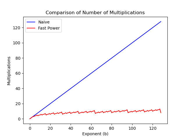
This should still be significantly faster than the naive method. We can plot modPow(5,b,9) for different values of \(b\) to see which is doing less work. Since each multiplication needs to be done on the processor, the less multiplications we do the faster the answer will be computed.

First, we can compare the fast and naive methods. This chart makes the savings in number of multiplications very obvious.

Fast vs Naive Method

We can also see how our estimated bounds worked out by plotting them. Since the naive method is so far off, it makes sense to focus on the plot without this version. This chart shows that the real number of multiplications always falls in between our two estimates. We can use these bounds to make estimates of the number of multiplications without always calculating them exactly.

Bound Estimates

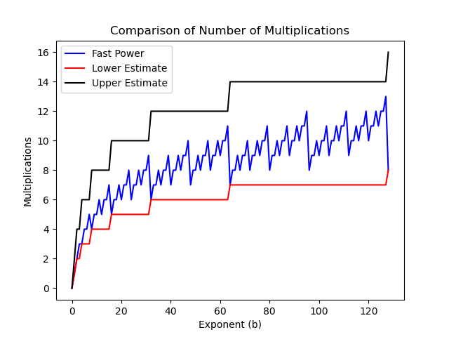
We can conclude that the runtime of this algorithm is \(O(\log_2(n))\).

Conclusion¶

The algorithm for fast powering uses drastically fewer multiplications. This will mean the algorithm will take less time. Every multiplication takes time to do, if we do less work it will take less time. In a future section, we will examine a formal method for comparing algorithms based on the number of operations they need to complete.

Algorithmic Foundations of Computer Science

Fast Modular Power

Contents