Merge Sort
Contents
Merge Sort
Overview
As a human, you would probably never use Bubble Sort or Insertion Sort in real life. If you had a large pile of papers to organize, working with them all at once is just to hard. Instead, you would break the problem up into smaller problems. You might organize your papers by topic or importance. Then sort the smaller piles.
The Merge Sort algorithm is inspired by this concept. Instead of sorting the entire array at once, we break it up into smaller parts. We sort the smaller parts. Then we merge the sorted arrays together to form larger arrays. Once all the values are merged together, the entire array is sorted.
Merge
The Merge Sort algorithm only works if we can efficiently merge two sorted lists. If we can’t do that, then there is no point in trying to sort. We need to be able to merge sorted lists efficiently.
Imagine you have two sets of numbers that are already sorted.
\( \begin{align} A=& [1,3,5] \\ B=& [2,4,8,10] \end{align} \)
What is the first value in the merged array? Well, we know A is sorted, so the smallest element in that array is at index \(0\). We also know \(B\) is sorted, which means the smallest element is at B[0]. That means there are only two values that could be the minimum. The minimum is either A[0] or B[0].
In this case, the minimum is A[0]=1. Once we determine that, we need the second smallest number. It is either B[0] or A[1]. Those are the remaining un-merged minimums.
We can build an algorithm for merging two sorted lists based on this concept. We don’t have to look at the entire list to find the next element in the merged list. We just need to compare the leading elements.
Merge Example
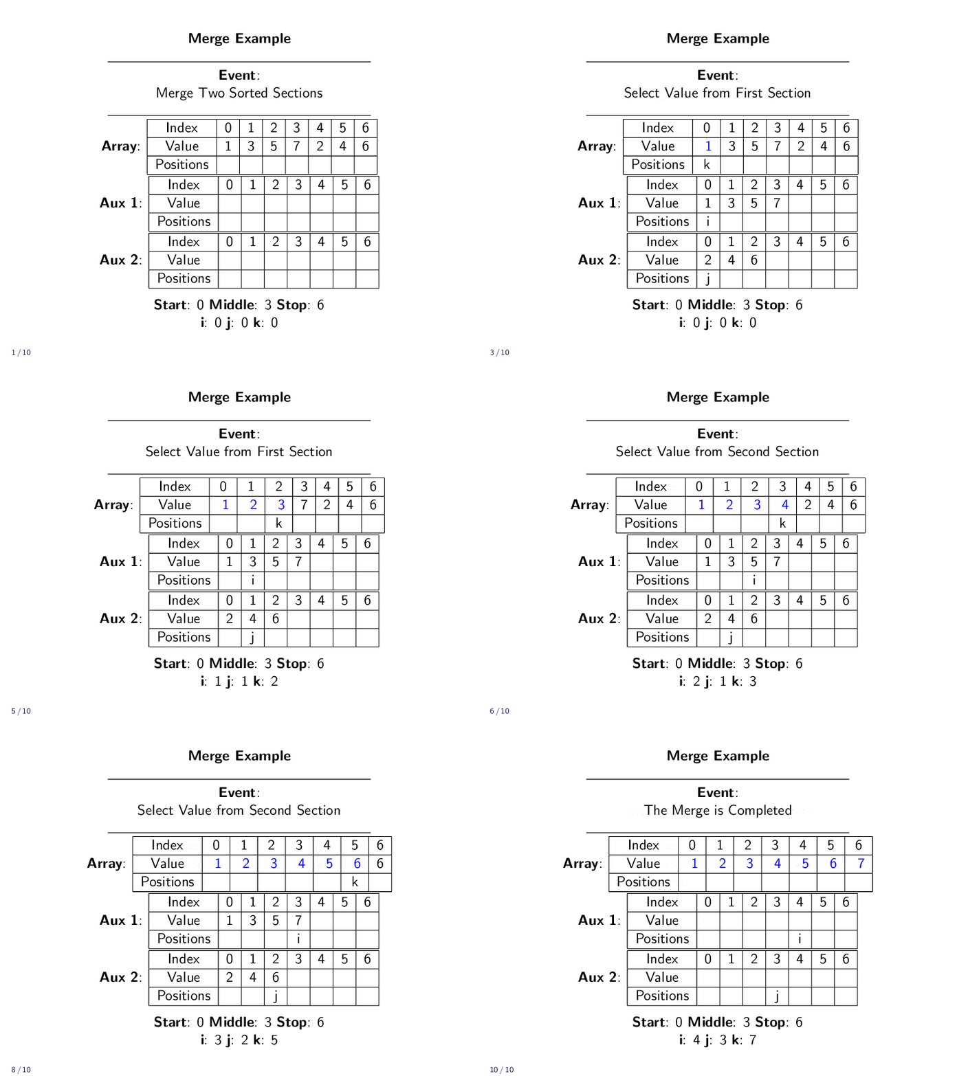
In practice, we don’t have two different lists. We are just merging together parts of an array. We use indexes to keep track of all the different positions.
kis the index in the array the value ends up iniis the current smallest unplaced value in the first sectionjis the current smallest unplaced value in the second section
If either section runs out of items, the all remaining elements just need to be copied over.

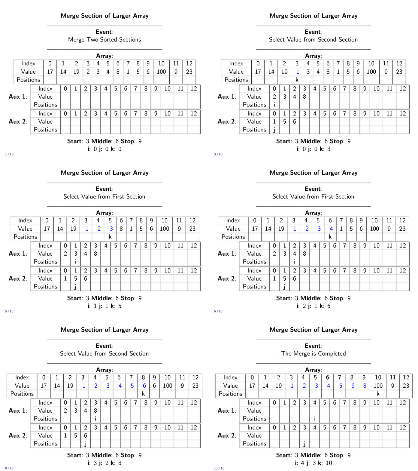
In practice, we won’t always be merging the entire array. We might only be merging a small part of a larger array. The next example shows only a fraction of the array being merged. The rest is left untouched.

Merge Implementation
To implement, we need to allocate two auxiliary arrays. One for the first section and one for the section. Our loop compares the first elements in each array. It copies the smaller one to primary array. Then it updates it counts to find the next smallest element.
It repeats until all elements have been correctly returned to the A array. It is important that we only copy the values we need into the auxiliary arrays. If we copy extra elements, the runtime of this algorithm will increase.
Function merge(array pointer A, int start, int middle, int stop)
    //Create Two AUX Arrays
    Let firstSectionSize = middle - start + 1
    Let firstSection = allocateArray(firstSectionSize)
    Let secondSectionSize = stop - middle
    Let secondSection = allocateArray(secondSectionSize)
    //Copy Elements in A from start to stop into Aux Arrays
    copyParts(A, firstSection, start, middle)
    copyParts(A, secondSection, middle+1, stop)
    //Set Variables
    Let i = 0
    Let j = 0
    //Loop Over Values
    For(k=start; k <= stop; k++)
        If i >= firstSectionSize then
            A[k] = secondSection[j]
            j = j + 1
        Else If j >= secondSectionSize then
            A[k] = firstSection[i]
            i = i + 1
        Else If secondSection[j] > firstSection[i] then
            A[k] = firstSection[i]
            i = i + 1
        Else
            A[k] = secondSection[j]
            j = j + 1
        End If
    End For
    //Clear Aux Data
    deleteArray(firstSection)
    deleteArray(secondSection)
End Function
Merge Analysis
We need to merge a total of \(n\) elements split between two sections of a larger array. We allocate two smaller arrays, but their total allocation is \(O(n)\) spaces. We then need to copy the values into the arrays. Again, between the two copies, we copy \(O(n)\) values.
Next, we have a loop. The loop iterates \(O(n)\) times. There are no nested loops.
Finally, we need to erase our auxiliary arrays. Keeping them around would waste memory. In the worst case, this causes the computer to actually delete all \(O(n)\) values.
Every step of this algorithm is \(O(n)\). The total runtime of the Merge algorithm is \(O(n)\).
The memory needed is also \(O(n)\). It needs the values to copy \(O(n)\) and the auxiliary space \(O(n)\). It also needs some constant amount of extra space for variables and the function definition.
The Merge algorithm is a linear time and linear space complexity algorithm.
Merge Sort Algorithm
The Merge Sort algorithm uses the Merge Algorithm. To sort, we divide the array in half. We merge the two halves using a recursive function call. Once the two halves are sorted, we merge them back together.
Merge Sort Example
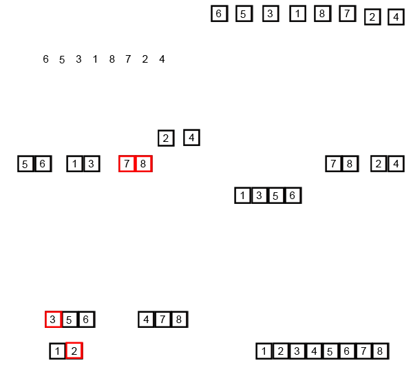
The following animation shows a full execution of the Merge Sort algorithm.

By Swfung8 - Own work, CC BY-SA 3.0, Link
Implementation
The implementation is recursive. We start with the entire array from 0 to size-1. The recursion repeats until start >= stop, which means there are no more elements to sort.
Each iteration of the recursion determines the middle of the array. Recursive calls sort the two halves. Then merge is called to combined the two halves.
//The MergeSort function gives the recursive
//call a consistent format with our other sorts
Function mergesort(array pointer A, int size)
    msort(A, 0, size-1)
End Function

//This function does the real merge sort
Function msort(array pointer A, int start, int stop)
    If start >= stop then
        Return
    End If
    Let middle = start + ((stop - start) / 2)
    msort(A, start, middle)
    msort(A, middle+1, stop)
    merge(A, start, middle, stop)
End Function
Merge Sort Analysis
The Merge Sort algorithm is recursive. It is easiest to analyze using a recursive formula.
\( \begin{align} T(n) =& \text{mergesort}(\text{First Half}) + \text{mergesort}(\text{Second Half}) + \text{merge}(\text{Both Halves}) \end{align} \)
We already determined that the Merge algorithm was \(O(n)\). The Merge Sort algorithm is a recursive one. We can write the formula as
\( \begin{align} T(n) =& T(n/2) + T(n/2) + n \\ =& 2T(n/2) + n \end{align} \)
We can use expansion to solve for a closed form of this recursion.
We expand the recursion to look for a pattern.
\( \begin{align} T(n) =& 2T(n/2) + n & \text{Iteration 1}\\ =& 2 \left( 2T(n/4) + n/2 \right) + n &\text{Expand} \\ =& 4T(n/4) + 2n & \text{Iteration 2} \\ =& 4 \left( 2T(n/8) + n/4 \right) + 2n &\text{Expand} \\ =& 8T(n/8) + 3n &\text{Iteration 3} \\ =& 8 \left( 2T(n/16) + n/8 \right) + 3n &\text{Expand} \\ =& 16T(n/16) + 4n &\text{Iteration 4} \end{align} \)
This expansion has a pattern. The \(k\)-th iteration will be
\( \begin{align} T(n) =& 2^k T(n/2^{k}) + kn \end{align} \)
When we get to \(T(1)\) the sort will only take \(O(1)\) operations. A array with one element is already sorted. It just takes a constant amount of work to realized the array is sorted.
When does it reach \(T(1) = T(n/2^k)\)?
\( \begin{align} 1 =& \frac{n}{2^k} \\ 2^k =& n \\ k =& \log_{2}(n) \end{align} \)
We can plug the stopping condition into the iteration formula.
\( \begin{align} T(n) =& 2^k T(n/2^{k}) + kn \\ =& 2^{\log_2(n)} T(n/2^{\log_{2}(n)}) + n \log_{2}(n) \\ =& nT(1) + n \log_2(n) \\ =& n \log_2(n) + n \\ =& O(n \log_{2}(n)) \end{align} \)
The Merge Sort algorithm’s runtime is \(O(n \log_{2} (n))\). This is the same runtime class as the theoretical perfect sorting algorithm. It may have a higher constant, but it has the same growth rate as the theoretically perfect solution.
The memory usage of Merge Sort is also \(O(n)\). The array is passed in and not part of Merge Sort’s memory usage. The temporary auxiliary array is needed. At any one time, there will only be one temporary array and it will be deleted before the next one is needed. This takes \(O(n)\) space. The function also has local variables and will make calls on the stack. In the worst case, the stack will also have \(O(n)\) function calls.
The memory usage of Merge Sort is \(O(n)\).
